More on ANOVA
| Site: | Saylor University |
| Course: | MA121: Introduction to Statistics |
| Book: | More on ANOVA |
| Printed by: | Guest user |
| Date: | Sunday, 21 June 2026, 9:28 AM |
Description
Introduction
Analysis of Variance (ANOVA) is a statistical method used to test differences between two or more means. It may seem odd that the technique is called "Analysis of Variance" rather than "Analysis of Means". As you will see, the name is appropriate because inferences about means are made by analyzing variance.
ANOVA is used to test general rather than specific differences among means. This can be seen best by example. In the case study "Smiles and Leniency," the effect of different types of smiles on the leniency shown to a person was investigated. Four different types of smiles (neutral, false, felt, miserable) were investigated. The chapter "All Pairwise Comparisons among Means" showed how to test differences among means. The results from the Tukey HSD test are shown in Table 1.
Table 1. Six Pairwise Comparisons.
| Comparison | Mi-Mj | Q | p |
|---|---|---|---|
| False - Felt | 0.46 | 1.65 | 0.649 |
| False - Miserable | 0.46 | 1.65 | 0.649 |
| False - Neutral | 1.25 | 4.48 | 0.010 |
| Felt - Miserable | 0.00 | 0.00 | 1.000 |
| Felt - Neutral | 0.79 | 2.83 | 0.193 |
| Miserable - Neutral | 0.79 | 2.83 | 0.193 |
Notice that the only significant difference is between the False and Neutral conditions.
ANOVA tests the non-specific null hypothesis that all four population means are equal. That is,
μfalse = μfelt = μmiserable = μneutral.
This non-specific null hypothesis is sometimes called the omnibus null hypothesis. When the omnibus null hypothesis is rejected, the conclusion is that at least one population mean is different from at least one other mean. However, since the ANOVA does not reveal which means are different from which, it offers less specific information than the Tukey HSD test. The Tukey HSD is therefore preferable to ANOVA in this situation. Some textbooks introduce the Tukey test only as a follow-up to an ANOVA. However, there is no logical or statistical reason why you should not use the Tukey test even if you do not compute an ANOVA.
You might be wondering why you should learn about ANOVA when the Tukey test is better. One reason is that there are complex types of analyses that can be done with ANOVA and not with the Tukey test. A second is that ANOVA is by far the most commonly-used technique for comparing means, and it is important to understand ANOVA in order to understand research reports.
Source: David M. Lane , https://onlinestatbook.com/2/analysis_of_variance/ANOVA.html![]() This work is in the Public Domain.
This work is in the Public Domain.
Video
Questions
Question 1 out of 3.
The omnibus null hypothesis when performing an analysis of variance is that there are differences between group means; however, no prediction is made concerning where the differences lie.
- True
- False
Question 2 out of 3.
Unlike t tests, an ANOVA may be used to test for differences among more than 2 groups.
- True
- False
Question 3 out of 3.
It is valid to do the Tukey HSD test without first finding a significant effect with an ANOVA.
- True
- False
Answers
-
False, the omnibus null hypothesis is that all population means are the same.
-
True, an analysis of variance (ANOVA) is most often used to determine if there are differences among 3 or more group means. However, when there are more than 2 groups, an ANOVA does not provide information regarding where the differences lie.
-
True, the Tukey HSD controls the Type I error rate and is valid without first running an ANOVA.
Analysis of Variance Designs
There are many types of experimental designs that can be analyzed by ANOVA. This section discusses many of these designs and defines several key terms used.
Factors and Levels
The section on variables defined an independent variable as a variable manipulated by the experimenter. In the case study "Smiles and Leniency," the effect of different types of smiles on the leniency shown to a person was investigated. Four different types of smiles (neutral, false, felt, and miserable) were shown. In this experiment, "Type of Smile" is the independent variable. In describing an ANOVA design, the term factor is a synonym of independent variable. Therefore, "Type of Smile" is the factor in this experiment. Since four types of smiles were compared, the factor "Type of Smile" has four levels.
An ANOVA conducted on a design in which there is only one factor is called a one-way ANOVA. If an experiment has two factors, then the ANOVA is called a two-way ANOVA. For example, suppose an experiment on the effects of age and gender on reading speed were conducted using three age groups (8 years, 10 years, and 12 years) and the two genders (male and female). The factors would be age and gender. Age would have three levels and gender would have two levels.
Between- and Within-Subjects Factors
In the "Smiles and Leniency" study, the four levels of the factor "Type of Smile" were represented by four separate groups of subjects. When different subjects are used for the levels of a factor, the factor is called a between-subjects factor or a between-subjects variable. The term "between subjects" reflects the fact that comparisons are between different groups of subjects.
In the "ADHD
Treatment" study, every subject was tested
with each of four dosage levels
(0, 0.15, 0.30, 0.60 mg/kg) of a drug. Therefore there was only
one group of subjects, and comparisons were not between different
groups of subjects but between conditions within the same subjects.
When the same subjects are used for the levels of a factor,
the factor is called a within-subjects factor or a within-subjects
variable. Within-subjects variables are sometimes referred
to as repeated-measures variables since
there are repeated measurements of the same subjects.
Multi-Factor Designs
It is common for designs to have more than one factor. For example, consider a hypothetical study of the effects of age and gender on reading speed in which males and females from the age levels of 8 years, 10 years, and 12 years are tested. There would be a total of six different groups as shown in Table 1.
Table 1. Gender x Age Design.
| Group | Gender | Age |
|---|---|---|
| 1 | Female | 8 |
| 2 | Female | 10 |
| 3 | Female | 12 |
| 4 | Male | 8 |
| 5 | Male | 10 |
| 6 | Male | 12 |
This design has two factors: age and gender. Age has three levels and gender has two levels. When all combinations of the levels are included (as they are here), the design is called a factorial design. A concise way of describing this design is as a Gender (2) x Age (3) factorial design where the numbers in parentheses indicate the number of levels. Complex designs frequently have more than two factors and may have combinations of between- and within-subjects factors.
Questions
Question 1 out of 4.
Fifty subjects are each tested in both a control condition and an experimental condition. This is an example of:
- a between-subjects design
- a within-subjects design
Question 2 out of 4.
The times it took each of 20 subjects to name a set of colored squares and to read a set of color names were recorded. This is an example of:
- a between-subjects design
- a within-subjects design
Question 3 out of 4.
Subjects are randomly assigned to either a drug condition or a placebo condition. This is an example of:
- a between-subjects design
- a within-subjects design
Question 4 out of 4.
In a Gender (2) x Treatment (6) factorial between-subjects design, the total number of separate groups is
Answers
-
This is a within-subjects design since each subject was tested in each condition.
-
This is a within-subjects design since each subject was tested in each condition.
-
This is a between-subjects design because each subject was tested in either one condition (drug) or another (placebo).
-
12. All combinations of Gender and Treatment would be in the design.
One-Factor ANOVA (Between Subjects)
This section shows how ANOVA can be used to analyze a one-factor between-subjects design. We will use as our main example the "Smiles and Leniency" case study. In this study, there were four conditions with 34 subjects in each condition. There was one score per subject. The null hypothesis tested by ANOVA is that the population means for all conditions are the same. This can be expressed as follows:

where H0 is the null
hypothesis and k is the number of conditions. In the "Smiles and
Leniency" study,  and the null hypothesis is
 .
.
If the null hypothesis is rejected, then it can be concluded that at least one of the population means is different from at least one other population mean.
Analysis of variance is a method
for testing differences among means by analyzing variance. The
test is based on two estimates of the population variance ") .
One estimate is called the mean square error
.
One estimate is called the mean square error  and is based
on differences among scores within the groups. estimates
and is based
on differences among scores within the groups. estimates  regardless
of whether the null hypothesis is true (the population means
are equal). The second estimate is called the mean square
between
regardless
of whether the null hypothesis is true (the population means
are equal). The second estimate is called the mean square
between  and is based on differences among the sample means. only estimates if
the population means are equal. If the population means are
not equal, then estimates a quantity larger than .
Therefore, if the is much larger than the , then the
population means are unlikely to be equal. On the other hand,
if the is about the same as , then the data are consistent
with the null hypothesis that the population means are equal.
and is based on differences among the sample means. only estimates if
the population means are equal. If the population means are
not equal, then estimates a quantity larger than .
Therefore, if the is much larger than the , then the
population means are unlikely to be equal. On the other hand,
if the is about the same as , then the data are consistent
with the null hypothesis that the population means are equal.
Before proceeding with the calculation of and
, it is important to consider the assumptions made by ANOVA:
- The populations have the same variance. This assumption is called the assumption of homogeneity of variance.
- The populations are normally distributed.
- Each value is sampled independently from each other value. This assumption requires that each subject provide only one value. If a subject provides two scores, then the values are not independent. The analysis of data with two scores per subject is shown in the section on within-subjects ANOVA later in this chapter.
These assumptions are the same as for a  test of differences between groups except that they apply
to two or more groups, not just to two groups.
test of differences between groups except that they apply
to two or more groups, not just to two groups.
The means and variances of the four groups in the "Smiles and Leniency" case study are shown in Table 1. Note that there are 34 subjects in each of the four conditions (False, Felt, Miserable, and Neutral).
Table 1. Means and Variances from the "Smiles and Leniency" Study.
| Condition | Mean | Variance |
|---|---|---|
| False | 5.3676 | 3.3380 |
| Felt | 4.9118 | 2.8253 |
| Miserable | 4.9118 | 2.1132 |
| Neutral | 4.1176 | 2.3191 |
Sample Sizes
 .
For these data, there are four groups of 34 observations. Therefore,
.
For these data, there are four groups of 34 observations. Therefore,
 and
and  .
. Computing
Recall that the assumption of homogeneity of variance
states that the variance within each of the populations ()
is the same.
This variance, ,
is the quantity estimated by and is computed as the mean
of the sample variances. For these data, the
is equal to 2.6489.
Computing
The formula for is based on the fact that
the variance of the sampling
distribution of the mean is

where  is the sample size of each group. Rearranging this formula,
we have
is the sample size of each group. Rearranging this formula,
we have

Therefore, if we knew the variance of the sampling
distribution of the mean, we could compute by
multiplying it by . Although we do not know the variance of the
sampling distribution of the mean, we can estimate it with the
variance of the sample means. For the leniency data, the variance
of the four sample means is 0.270. To estimate ,
we multiply the variance of the sample means (0.270) by n (the
number of observations in each group, which is 34). We find
that = 9.179.
To sum up these steps:
- Compute the means.
- Compute the variance of the means.
- Multiply the variance of the means by .
Recap
If the population means are equal, then both
and are estimates of and
should therefore be about the same. Naturally, they will not
be exactly the same since they are just estimates and are based
on different aspects of the data: The is computed from the
sample means and the is computed from the sample variances.
If the population means are not equal, then
will still estimate because
differences in population means do not affect variances. However,
differences in population means affect since differences
among population means are associated with differences among
sample means. It follows that the larger the differences among
sample means, the larger the . In
short, estimates whether or not the population means are equal, whereas
estimates only
when
the population means are equal and estimates a larger quantity
when they are not equal.
Comparing and
The critical step in an ANOVA is comparing
and . Since estimates a larger quantity than only
when the population means are not equal, a finding of a larger
than an is a sign that the population means are not
equal. But since could be larger than by chance even
if the population means are equal, must be much larger than
in order to justify the conclusion that the population means
differ. But how much larger must be? For the "Smiles and
Leniency" data, the and are 9.179 and 2.649, respectively.
Is that difference big enough? To answer, we would need to know
the probability of getting that big a difference or a bigger
difference if the population means were
all equal. The mathematics necessary to
answer this question were worked out by the statistician R.
Fisher. Although Fisher's original formulation took a slightly
different form, the standard method for determining the probability
is based on the ratio of to . This ratio is named after
Fisher and is called the  ratio.
For these
data, the ratio is
 .
.
Therefore, the is 3.465 times
higher than
. Would this have been likely to happen if all the
population
means were equal? That depends on the sample size. With
a small sample size, it would not be too surprising because results
from small samples are unstable. However, with a very large sample, the
and
are almost always about the same, and an F ratio of
3.465
or larger would be very unusual. Figure 1 shows the sampling
distribution of F
for the sample size in the "Smiles and Leniency" study. As you
can see, it has a positive skew.
Figure 1. Distribution of .
From Figure 1, you can see that F ratios of 3.465 or above are unusual occurrences. The area to the right of 3.465 represents the probability of an F that large or larger and is equal to 0.018. In other words, given the null hypothesis that all the population means are equal, the probability value is 0.018 and therefore the null hypothesis can be rejected. The conclusion that at least one of the population means is different from at least one of the others is justified.
The shape of the F distribution
depends on the sample size. More precisely, it depends on two
degrees
of freedom ( ) parameters: one for the numerator ()
and one for the denominator (). Recall that the degrees
of freedom for an estimate of variance is equal to
the number
of observations minus one. Since the is the variance
of
) parameters: one for the numerator ()
and one for the denominator (). Recall that the degrees
of freedom for an estimate of variance is equal to
the number
of observations minus one. Since the is the variance
of  means, it has
  . The is an average of variances, each
with
. The is an average of variances, each
with  . Therefore, the for is
  = N - k") , where is
the total number of observations, is the number of observations in
each group, and k is the number of groups. To summarize:
, where is
the total number of observations, is the number of observations in
each group, and k is the number of groups. To summarize:


For the "Smiles and Leniency" data,


The distribution calculator shows that  .
.
One-Tailed or Two?
Is the probability value from an ratio a one-tailed or a two-tailed probability? In the literal sense, it is a one-tailed
probability since, as you can see in Figure 1, the probability
is the area in the right-hand tail of the distribution.
However, the ratio is sensitive to any pattern of differences
among means. It is, therefore, a test of a two-tailed hypothesis
and is best considered a two-tailed test.
Relationship to the t test
Since an ANOVA and an independent-groups t test can both test the difference between two means, you might be wondering which one to use. Fortunately, it does not matter since the results will always be the same. When there are only two groups, the following relationship between F and t will always hold:
 = t^2(df)")
where  is the degrees of freedom for
the denominator of the test and is the degrees of freedom
for the test. will always equal .
is the degrees of freedom for
the denominator of the test and is the degrees of freedom
for the test. will always equal .
Sources of Variation
Why do scores in an experiment differ from one another? Consider the scores of two subjects in the "Smiles and Leniency" study: one from the "False Smile" condition and one from the "Felt Smile" condition. An obvious possible reason that the scores could differ is that the subjects were treated differently (they were in different conditions and saw different stimuli). A second reason is that the two subjects may have differed with regard to their tendency to judge people leniently. A third is that, perhaps, one of the subjects was in a bad mood after receiving a low grade on a test. You can imagine that there are innumerable other reasons why the scores of the two subjects could differ. All of these reasons except the first (subjects were treated differently) are possibilities that were not under experimental investigation and, therefore, all of the differences (variation) due to these possibilities are unexplained. It is traditional to call unexplained variance error even though there is no implication that an error was made. Therefore, the variation in this experiment can be thought of as being either variation due to the condition the subject was in or due to error (the sum total of all reasons the subjects' scores could differ that were not measured).
One of the important characteristics of ANOVA is that it partitions the variation into its various sources. In ANOVA, the term sum of squares (SSQ) is used to indicate variation. The total variation is defined as the sum of squared differences between each score and the mean of all subjects. The mean of all subjects is called the grand mean and is designated as GM. (When there is an equal number of subjects in each condition, the grand mean is the mean of the condition means.) The total sum of squares is defined as
^{2}")
which means to take each score, subtract
the grand mean from it, square the difference, and then sum
up these squared values. For the "Smiles and Leniency" study,
^{2} = 377.19") .
.
The sum of squares condition is calculated as shown below.
![S S Q_{\text {condition }}=\mathrm{n}\left[\left(\mathrm{M}_{1}-G M\right)^{2}+\left(\mathrm{M}_{2}-G M\right)^{2}+\ldots+\left(\mathrm{M}_{\mathrm{k}}-G M\right)^{2}\right]](https://dev.sylr.org/filter/tex/pix.php/98a702d9481d91f6da16038d85f843c3.gif "S S Q_{\text {condition }}=\mathrm{n}\left[\left(\mathrm{M}_{1}-G M\right)^{2}+\left(\mathrm{M}_{2}-G M\right)^{2}+\ldots+\left(\mathrm{M}_{\mathrm{k}}-G M\right)^{2}\right]")
where n is the number of scores in each group,
is the number of groups,  is
the mean for Condition 1,
is
the mean for Condition 1,  is the
mean for Condition 2, and
is the
mean for Condition 2, and  is the
mean for Condition k. For the Smiles and Leniency study, the
values are:
is the
mean for Condition k. For the Smiles and Leniency study, the
values are:
![SSQ_{condition} =
34[(5.37-4.83)^2 +
(4.91-4.83)^2 + (4.91-4.83)^2 + (4.12-4.83)^2]](https://dev.sylr.org/filter/tex/pix.php/bc40bdc9e878795b232d71041256d34e.gif "SSQ_{condition} =
34[(5.37-4.83)^2 +
(4.91-4.83)^2 + (4.91-4.83)^2 + (4.12-4.83)^2]")

If there are unequal sample sizes, the only change is that the following formula is used for the sum of squares condition:
^{2}+\mathrm{n}_{2}\left(\mathrm{M}_{2}-G M\right)^{2}+\ldots+\mathrm{n}_{\mathrm{k}}\left(\mathrm{M}_{\mathrm{k}}-G M\right)^{2}")
where  is the sample
size of the ith condition.
is the sample
size of the ith condition.  is computed the same way
as shown above.
is computed the same way
as shown above.
The sum of squares error is the sum of the squared deviations of each score from its group mean. This can be written as
^{2}+\sum\left(X_{\mathrm{i} 2}-M_{2}\right)^{2}+\ldots+\sum\left(X_{\mathrm{ik}}-M_{\mathrm{k}}\right)^{2}")
where  is the
ith score in group 1 and is the
mean for group 1,
is the
ith score in group 1 and is the
mean for group 1,  is the ith
score in group 2 and is the mean
for group 2, etc. For the "Smiles and Leniency" study, the
means are: 5.368, 4.912, 4.912, and 4.118. The SSQerror is
therefore:
is the ith
score in group 2 and is the mean
for group 2, etc. For the "Smiles and Leniency" study, the
means are: 5.368, 4.912, 4.912, and 4.118. The SSQerror is
therefore:
(2.5-5.368)2 + (5.5-5.368)2 + ... + (6.5-4.118)2 = 349.65
The sum of squares error can also be computed by subtraction:


Therefore, the total sum of squares of 377.19
can be partitioned into  (27.53)
and
(27.53)
and  (349.66).
Once the sums of squares have been computed,
the mean squares ( and ) can be computed easily. The
formulas are:

where dfn is the degrees of freedom numerator
and is equal to  .
.

which is the same value of obtained
previously (except for rounding error). Similarly,

where dfd is the degrees of freedom for
the denominator and is equal to  .
.


which is the same as obtained previously (except for rounding error). Note that the dfd is often called the dfe for degrees of freedom error.
The Analysis of Variance Summary Table shown
below is a convenient way to summarize the partitioning of
the variance. The rounding errors have been corrected.
Table 2. ANOVA Summary Table.
| Source | df | SSQ | MS | F | p |
|---|---|---|---|---|---|
| Condition | 3 | 27.5349 | 9.1783 | 3.465 | 0.0182 |
| Error | 132 | 349.6544 | 2.6489 | ||
| Total | 135 | 377.1893 |
The first column shows the sources of variation, the second
column shows the degrees of freedom, the third shows the
sums of squares, the fourth shows the mean squares, the fifth shows the ratio, and the last
shows the probability value. Note that the mean squares
are always the sums of squares divided by degrees of freedom.
The and  are relevant only to Condition. Although the
mean square total could be computed by dividing the sum
of squares by the degrees of freedom, it is generally not
of much interest and is omitted here.
are relevant only to Condition. Although the
mean square total could be computed by dividing the sum
of squares by the degrees of freedom, it is generally not
of much interest and is omitted here.
Formatting Data for Computer Analysis
Most computer programs that compute ANOVAs require your data to be in a specific form. Consider the data in Table 3.
Table 3. Example Data.
| Group 1 | Group 2 | Group 3 |
|---|---|---|
| 3 | 2 | 8 |
| 4 | 4 | 5 |
| 5 | 6 | 5 |
Table 4. Reformatted Data.
| G | Y |
|---|---|
| 1 | 3 |
| 1 | 4 |
| 1 | 5 |
| 2 | 2 |
| 2 | 4 |
| 2 | 6 |
| 3 | 8 |
| 3 | 5 |
| 3 | 5 |
R code
Make sure to put the data files in the default directory.
leniency = read.csv(file = "leniency.CSV")
leniency.f <- factor(leniency$smile, levels = c("1", "2", "3", "4"))
leniency_model <- lm(leniency~ leniency.f, data = leniency)
summary(aov(leniency_model))
             Df Sum Sq Mean Sq F value Pr(>F)
leniency.f    3   27.5   9.178   3.465 0.0182
Residuals   132  349.7   2.649
Questions
Question 1 out of 20.
Unlike t tests, an ANOVA uses both differences between group means and differences within groups to determine whether or not the differences are significant.
- True
- False
Question 2 out of 20.
The "Smiles and Leniency" study uses a between-subjects design. The four types of
smiles (false, felt, miserable, and neutral) are the four levels of one factor.
Question 3 out of 20.
If an experiment seeks to investigate the acquisition of skill over multiple sessions of practice, which of the following best describes the comparison of the subjects?
- Within-subjects
- Between-subjects
- Cannot be determined with the given information
Question 4 out of 20.
These values are from three independent groups. What is the p value in a one-way ANOVA? (If you are using a program, make sure to reformat the data as described.)
 G1	 G2	 G3
 54	 48	 61
 41	 44	 54
 65	 42	 51
 61	 64	 45
 53	 38	 30
 60	 63	 42
 58	 58	 34
 49	 59	 49
Question 5 out of 20.
These values are from three independent groups. What is the F in a one-way ANOVA? (If you are using a program, make sure to reformat the data as described.)
 G1	 G2	 G3
 60	 41	 68
 57	 50	 67
 47	 42	 57
 53	 39	 49
 80	 51	 47
 54	 54	 54
 41	 43	 48
Question 6 out of 20.
The table shows the means and variances from 5 experimental conditions. Compute the variance of the means.
Mean	Variance
  4.5	  1.33
  7.2	  0.98
  3.4	  1.03
  9.1	  0.78
  1.2	  0.56
Question 7 out of 20.
Compute the MSB based on the variance of the means. (These are the same values as previously shown.) The sample size for each mean is 10.
Mean	Variance
  4.5	  1.33
  7.2	  0.98
  3.4	  1.03
  9.1	  0.78
  1.2	  0.56
Question 8 out of 20.
Find the MSE by computing the mean of the variances.
Mean	Variance
  4.5	  1.33
  7.2	  0.98
  3.4	  1.03
  9.1	  0.78
  1.2	  0.56
Question 9 out of 20.
Which best describes the assumption of homogeneity of variance?
- The populations are both normally distributed to the same degree.
- The between and within population variances are approximately the same.
- The variances in the populations are equal.
Question 10 out of 20.
When performing a one-factor ANOVA (between-subjects), it is important that each subject only provide a single value. If a subject were to provide more than one value, the independence of each value would be lost and the test provided by an ANOVA would not be valid.
- True
- False
Question 11 out of 20.
If the MSE and MSB are approximately the same, it is highly likely that population means are different.
- True
- False
Question 12 out of 20.
You want to make a strong case that the different groups you have tested come from populations with different means. Your case is strongest when:
- MSE/MSB is high.
- MSE/MSB = 1.
- MSB/MSE is low.
- MSB/MSE is high.
Question 13 out of 20.
Why can't an F ratio be below 0?
- Neither MSB nor MSE can ever be a negative value.
- MSB is never less than 1.
- MSE is never less than 1.
Question 14 out of 20.
Consider an experiment in which there are 7 groups and within each group there are 15 participants. What is the degrees of freedom for the numerator (between)?
Question 15 out of 20.
Consider an experiment in which there are 7 groups and within each group there are 15 participants. What is the degrees of freedom for the denominator (within)?
Question 16 out of 20.
The F distribution has a:
- positive skew
- no skew
- negative skew
Question 17 out of 20.
An independent-groups t test with 12 degrees of freedom was conducted and the value of t was 2.5. What would the F be in a one-factor ANOVA?
Question 18 out of 20.
If the sum of squares total were 100 and the sum of squares condition were 80, what would the sum of squares error be?
Question 19 out of 20.
If the sum of squares total were 100 and the sum of squares condition were 80 in an experiment with 3 groups and 8 subjects per group, what would the F ratio be?
Question 20 out of 20.
If a t test of the difference between
means of two independent groups found a t of 2.5, what would be the
value of F in a one-way ANOVA?
Answers
-
False, both t tests and ANOVAs use both. In a t test, the difference between means is in the numerator and the denominator is based on differences within groups. In an ANOVA, the variance of the group means (multiplied by n) is the numerator. The denominator is based on differences within groups.
-
This is correct. These are the four levels of the variable "Type of Smile".
-
This is a within-subjects design since subjects are tested multiple times. In a between-subjects design each subject provides only one score.
-
p = 0.3562
-
F = 1.3057
-
variance of the means = 9.717
-
Multiply the variance of the means by the n of 10. The result is 97.17.
-
.936
-
Homogeneity of variance is the assumption that the variances in the populations are equal.
-
True. When a subject provides more than one data point, the values are not independent, thus violating one of the assumptions of between-subjects ANOVA.
-
False. If the null hypothesis that all of the population means are equal is true, then both MSB and MSE estimate the same quantity.
-
When the population means differ, MSB estimates a quantity larger than does MSE. A high ratio of MSB to MSE is evidence that the population means are different.
-
F is defined as MSB/MSE. Since both MSB and MSE are variances and negative variance is impossible, an F score can never be negative.
-
k-1 = 7-1 = 6
-
N-k = 105-7 = 98
-
The F distribution has a long tail to the right which means it has a positive skew.
-
F equals t2 = 6.25.
-
Sum of squares total equals sum of squares condition + sum of squares error.
-
Divide sums of squares by degrees of freedom to get mean squares. Then divide MSB by MSE to get F which equals 42.
-
F = t2
One-way ANOVA Demonstration
Instructions
This simulation demonstrates the partitioning of sums of squares in analysis of variance (ANOVA). Initially, you see a display of the first sample dataset. There are three groups of subjects, and four subjects per group. Each score is represented by a small black rectangle; the mean is represented as a red horizontal line. The values range from 0 to 10. The Y-axis ticks represent values of 0, 2.25, 5, 7.75, and 10. The means of the three groups are 2.50, 5.50, and 8.50.
The table in the lower left-hand portion of the window displays, for each group, the sample size, the mean, the sum of squared deviations of individual scores from the mean, and the squared difference between the group mean and the grand mean multiplied by the sample size. The bottom row shows the sums of these quantities. The sum of the last column is the sums of squares between while the sum of the second-to-last column is the sum of squares within. The ANOVA summary table based on these values is shown to the right. The sum of squares between and within are depicted graphically above the ANOVA summary table.
You can choose other datasets using the pop-up menu. You can also enter your own data by clicking on the data display. If you click in a blank area, an new data point is created (if you hold the mouse down after you click you can position the point by moving the mouse). You can modify the data by clicking on a point and moving it to another location. Finally, you can delete a data point by dragging it outside the colored region.
-
Notice how the sum of squares total is divided up into the sum of squared differences of each score from its group mean and the sum of squared differences of the group mean from the grand mean (GM: the mean of all data). Keep in mind that differences of group means from the grand mean have to be multiplied by the sample size.
-
Add a few data points by clicking and note the effects on the sums of squares. Notice that if the points are far from the group mean then the sum of squares within increases greatly.
-
Choose dataset 2. Notice that the means are very different and the data points are all near their group mean. This results in a large sum of squares between and a small sum of squares within.
-
Look at data set 4 which is similar but has more subjects.
-
Look at dataset 6 for which the group means are all the same. Note the value of the sum of squares between.
-
Choose "blank dataset" and enter your own data.
Illustrated Instructions
The video demonstration increases the mean of group 1 by dragging the individual points in the group. Notice how the statistics update as the points are moved.
Within-Subjects ANOVA
Within-subjects factors involve comparisons of the same subjects under different conditions. For example, in the "ADHD Treatment" study, each child's performance was measured four times, once after being on each of four drug doses for a week. Therefore, each subject's performance was measured at each of the four levels of the factor "Dose". Note the difference from between-subjects factors for which each subject's performance is measured only once and the comparisons are among different groups of subjects. A within-subjects factor is sometimes referred to as a repeated-measures factor since repeated measurements are taken on each subject. An experimental design in which the independent variable is a within-subjects factor is called a within-subjects design.
Advantage of Within-Subjects Designs
One-Factor Designs
Let's consider how to analyze the data from the "ADHD Treatment" case study. These data consist of the scores of 24 children with ADHD on a delay of gratification (DOG) task. Each child was tested under four dosage levels. For now, we will be concerned only with testing the difference between the mean in the placebo condition (the lowest dosage, D0) and the mean in the highest dosage condition (D60). The details of the computations are relatively unimportant since they are almost universally done by computers. Therefore we jump right to the ANOVA Summary table shown in Table 1.
Table 1. ANOVA Summary Table.
| Source | df | SSQ | MS | F | p |
|---|---|---|---|---|---|
| Subjects | 23 | 5781.98 | 251.39 | ||
| Dosage | 1 | 295.02 | 295.02 | 10.38 | 0.004 |
| Error | 23 | 653.48 | 28.41 | ||
| Total | 47 | 6730.48 |
The first source of variation, "Subjects," refers to the differences among subjects. If all the subjects had exactly the same mean (across the two dosages), then the sum of squares for subjects would be zero; the more subjects differ from each other, the larger the sum of squares subjects.
Dosage refers to the differences between the two dosage levels. If the means for the two dosage levels were equal, the sum of squares would be zero. The larger the difference between means, the larger the sum of squares.
The error reflects the degree to which the
effect of dosage is different for different subjects. If subjects all
responded very similarly to the drug, then the error would be very low.
For example, if all subjects performed moderately better with the high
dose than they did with the placebo, then the error would be low. On the
other hand, if some subjects did better with the placebo while others
did better with the high dose, then the error would be high. It should
make intuitive sense that the less consistent the effect of dosage, the
larger the dosage effect would have to be in order to be significant.
The degree to which the effect of dosage differs depending on the
subject is the Subjects  Dosage interaction. Recall that an interaction
occurs when the effect of one variable differs depending on the level
of another variable. In this case, the size of the error term is the
extent to which the effect of the variable "Dosage" differs depending on
the level of the variable "Subjects". Note that each subject is a
different level of the variable "Subjects".
Dosage interaction. Recall that an interaction
occurs when the effect of one variable differs depending on the level
of another variable. In this case, the size of the error term is the
extent to which the effect of the variable "Dosage" differs depending on
the level of the variable "Subjects". Note that each subject is a
different level of the variable "Subjects".
Other portions of the summary table have the same
meaning as in between-subjects ANOVA. The F for dosage is the
mean square for dosage divided by the mean square error. For these
data, the is significant with  . Notice that this F
test is equivalent to the t test
for correlated pairs, with
. Notice that this F
test is equivalent to the t test
for correlated pairs, with  .
.
Table 2 shows the ANOVA Summary Table when all four
doses are included in the analysis. Since there are now four dosage
levels rather than two, the df for dosage is three rather than
one. Since the error is the Subjects Dosage interaction, the
df for error is the df for "Subjects" (23) times the df for Dosage
(3) and is equal to 69.
Table 2. ANOVA Summary Table.
| Source | df | SSQ | MS | F | p |
|---|---|---|---|---|---|
| Subjects | 23 | 9065.49 | 394.15 | ||
| Dosage | 3 | 557.61 | 185.87 | 5.18 | 0.003 |
| Error | 69 | 2476.64 | 35.89 | ||
| Total | 95 | 12099.74 |
Carryover Effects
Often performing in one condition affects performance in a subsequent condition in such a way as to make a within-subjects design impractical. For example, consider an experiment with two conditions. In both conditions subjects are presented with pairs of words. In Condition A, subjects are asked to judge whether the words have similar meaning whereas in Condition B, subjects are asked to judge whether they sound similar. In both conditions, subjects are given a surprise memory test at the end of the presentation. If Condition were a within-subjects variable, then there would be no surprise after the second presentation and it is likely that the subjects would have been trying to memorize the words.
Not all carryover effects cause such serious problems. For example, if subjects get fatigued by performing a task, then they would be expected to do worse on the second condition they were in. However, as long as the order of presentation is counterbalanced so that half of the subjects are in Condition A first and Condition B second, the fatigue effect itself would not invalidate the results, although it would add noise and reduce power. The carryover effect is symmetric in that having Condition A first affects performance in Condition B to the same degree that having Condition B first affects performance in Condition A.
Asymmetric carryover effects cause more serious
problems. For example, suppose performance in Condition B were
much better if preceded by Condition A, whereas performance in
Condition A was approximately the same regardless of whether it
was preceded by Condition B. With this kind of carryover effect,
it is probably better to use a between-subjects
design.
One between- and one within-subjects factor
In the "Stroop Interference" case study, subjects performed three tasks: naming colors, reading color words, and naming the ink color of color words. Some of the subjects were males and some were females. Therefore, this design had two factors: gender and task. The ANOVA Summary Table for this design is shown in Table 3.
Table 3. ANOVA Summary Table for Stroop Experiment.
| Source | df | SSQ | MS | F | p |
|---|---|---|---|---|---|
| Gender | 1 | 83.32 | 83.32 | 1.99 | 0.165 |
| Error | 45 | 1880.56 | 41.79 | ||
| Task | 2 | 9525.97 | 4762.99 | 228.06 | <0.001 |
| Gender x Task | 2 | 55.85 | 27.92 | 1.34 | 0.268 |
| Error | 90 | 1879.67 | 20.89 |
The computations for the sums of squares will not be covered since computations are normally done by software. However, there are some important things to learn from the summary table. First, notice that there are two error terms: one for the between-subjects variable Gender and one for both the within-subjects variable Task and the interaction of the between-subjects variable and the within-subjects variable. Typically, the mean square error for the between-subjects variable will be higher than the other mean square error. In this example, the mean square error for Gender is about twice as large as the other mean square error.
The degrees of freedom for the between-subjects variable is equal to the number of levels of the between-subjects variable minus one. In this example, it is one since there are two levels of gender. Similarly, the degrees of freedom for the within-subjects variable is equal to the number of levels of the variable minus one. In this example, it is two since there are three tasks. The degrees of freedom for the interaction is the product of the degrees of freedom for the two variables. For the Gender x Task interaction, the degrees of freedom is the product of degrees of freedom Gender (which is 1) and the degrees of freedom Task (which is 2) and is equal to 2.
Assumption of Sphericity
Within-subjects ANOVA makes a restrictive assumption about the variances and the correlations among the dependent variables. Although the details of the assumption are beyond the scope of this book, it is approximately correct to say that it is assumed that all the correlations are equal and all the variances are equal. Table 4 shows the correlations among the three dependent variables in the "Stroop Interference" case study.
Table 4. Correlations Among Dependent Variables.
| word reading | color naming | interference | |
|---|---|---|---|
| word reading | 1 | 0.7013 | 0.1583 |
| color naming | 0.7013 | 1 | 0.2382 |
| interference | 0.1583 | 0.2382 | 1 |
Note that the correlation between the word reading and the color naming variables of 0.7013 is much higher than the correlation between either of these variables with the interference variable. Moreover, as shown in Table 5, the variances among the variables differ greatly.
Table 5. Variances.
| Variable | Variance |
|---|---|
| word reading | 15.77 |
| color naming | 13.92 |
| interference | 55.07 |
Naturally the assumption of sphericity, like
all assumptions, refers to populations not samples. However, it
is clear from these sample data that the assumption is not met
in the population.
Consequences of Violating the Assumption of Sphericity
Although ANOVA is robust to most violations of its assumptions, the assumption of sphericity is an exception: Violating the assumption of sphericity leads to a substantial increase in the Type I error rate. Moreover, this assumption is rarely met in practice. Although violations of this assumption had at one time received little attention, the current consensus of data analysts is that it is no longer considered acceptable to ignore them.
Approaches to Dealing with Violations of Sphericity
If an effect is highly significant, there is a conservative test that can be used to protect against an inflated Type I error rate. This test consists of adjusting the degrees of freedom for all within-subjects variables as follows: The degrees of freedom numerator and denominator are divided by the number of scores per subject minus one. Consider the effect of Task shown in Table 3. There are three scores per subject and therefore the degrees of freedom should be divided by two. The adjusted degrees of freedom are:
(2)(1/2) = 1 for the numerator and
(90)(1/2) = 45 for the denominator
The probability value is obtained using the F probability calculator with the new degrees of freedom parameters. The probability of an F of 228.06 or larger with 1 and 45 degrees of freedom is less than 0.001. Therefore, there is no need to worry about the assumption violation in this case.
Possible violation of sphericity does make a difference in the interpretation of the analysis shown in Table 2. The probability value of an F of 5.18 with 1 and 23 degrees of freedom is 0.032, a value that would lead to a more cautious conclusion than the p value of 0.003 shown in Table 2.
The correction described above is very conservative and should only be used when, as in Table 3, the probability value is very low. A better correction, but one that is very complicated to calculate, is to multiply the degrees of freedom by a quantity called ε (the Greek letter epsilon). There are two methods of calculating ε. The correction called the Huynh-Feldt (or H-F) is slightly preferred to the one called the Greenhouse-Geisser (or G-G), although both work well. The G-G correction is generally considered a little too conservative.
A final method for dealing with violations of sphericity is to use a multivariate approach to within-subjects variables. This method has much to recommend it, but it is beyond the scope of this text.
Questions
Question 1 out of 5.
Which of the following represent within-subjects variables?
- Age: Subjects of four different ages were used in the experiment.
- Trial: Each subject had three trials on the task and their score was recorded for each trial.
- Dose: Each subject was tested under each of five dosage levels.
- Day: Each subject was tested once a day for four days.
- Intensity: Each subject was randomly assigned to one of five intensity levels.
Question 2 out of 5.
Differences among subjects in overall performance constitute a source of error for
- between-subjects variables
- within-subjects variables
Question 3 out of 5.
Sphericity is an assumption made in
- between-subjects designs
- within-subjects designs
Question 4 out of 5.
Violating the assumption of sphericity:
- leads to a higher Type I error rate
- rarely has a meaningful effect on the Type I error rate
- decreases the Type I error rate
Question 5 out of 5.
Subjects were each tested under three conditions: quiet, noise, music. What is the F ratio in an ANOVA?
 quiet	 noise	 music
 49	 43	 80
 33	 56	 55
 39	 60	 77
 57	 41	 50
 69	 75	 60
 43	 50	 60
 40	 74	 79
 62	 49	 73
 60	 58	 57
 35	 65	 59
Answers
-
Trial, Dose, and Day. If different groups are used for each condition, then the variable is a between-subjects variable; if the same subjects are tested in each condition, then the variable is a within-subjects variable.
-
For between-subjects variables, differences among subjects are error. For within-subjects variables, each subject's performance in one condition is compared to his or her performance in another condition. Therefore, overall differences are not a source of error.
-
The assumption has to do with correlations among scores, which is not applicable in between-subjects designs since subjects have only one score.
-
Violating the assumption increases the Type I error rate, sometimes substantially.
-
0.049
Multi-Factor Between-Subjects Designs
Basic Concepts and Terms
In the "Bias Against Associates of the Obese" case study, the researchers were interested in whether the weight of a companion of a job applicant would affect judgments of a male applicant's qualifications for a job. Two independent variables were investigated: (1) whether the companion was obese or of typical weight and (2) whether the companion was a girlfriend or just an acquaintance. One approach could have been to conduct two separate studies, one with each independent variable. However, it is more efficient to conduct one study that includes both independent variables. Moreover, there is a much bigger advantage than efficiency for including two variables in the same study: it allows a test of the interaction between the variables. There is an interaction when the effect of one variable differs depending on the level of a second variable. For example, it is possible that the effect of having an obese companion would differ depending on the relationship to the companion. Perhaps there is more prejudice against a person with an obese companion if the companion is a girlfriend than if she is just an acquaintance. If so, there would be an interaction between the obesity factor and the relationship factor.There are three effects of interest in this experiment:
- Weight: Are applicants judged differently depending on the weight of their companion?
- Relationship: Are applicants judged differently depending on their relationship with their companion?
- Weight x Relationship Interaction: Does the effect of weight differ depending on the relationship with the companion?
The first two effects (Weight and Relationship) are both main effects. A main effect of an independent variable is the effect of the variable averaging over the levels of the other variable(s). It is convenient to talk about main effects in terms of marginal means. A marginal mean for a level of a variable is the mean of the means of all levels of the other variable. For example, the marginal mean for the level "Obese" is the mean of "Girlfriend Obese" and "Acquaintance Obese". Table 1 shows that this marginal mean is equal to the mean of 5.65 and 6.15, which is 5.90. Similarly, the marginal mean for the level "Typical" is the mean of 6.19 and 6.59, which is 6.39. The main effect of Weight is based on a comparison of these two marginal means. Similarly, the marginal means for "Girlfriend" and "Acquaintance" are 5.92 and 6.37.
Table 1. Means for All Four Conditions.
| Companion Weight | ||||
|---|---|---|---|---|
| Obese | Typical | Marginal Mean | ||
| Relationship | Girlfriend | 5.65 | 6.19 | 5.92 |
| Acquaintance | 6.15 | 6.59 | 6.37 | |
| Marginal Mean | 5.90 | 6.39 | ||
In contrast to a main effect, which is the effect of a variable averaged across levels of another variable, the simple effect of a variable is the effect of the variable at a single level of another variable. The simple effect of Weight at the level of "Girlfriend" is the difference between the "Girlfriend Typical" and the "Girlfriend Obese" conditions. The difference is 6.19-5.65 = 0.54. Similarly, the simple effect of Weight at the level of "Acquaintance" is the difference between the "Acquaintance Typical" and the "Acquaintance Obese" conditions. The difference is 6.59-6.15 = 0.44.
Recall that there is an interaction when the effect of one variable differs depending on the level of another variable. This is equivalent to saying that there is an interaction when the simple effects differ. In this example, the simple effects of weight are 0.54 and 0.44. As shown below, these simple effects are not significantly different.
Tests of Significance
The important questions are not whether there are main effects and interactions in the sample data. Instead, what is important is what the sample data allow you to conclude about the population. This is where Analysis of Variance comes in. ANOVA tests main effects and interactions for significance. An ANOVA Summary Table for these data is shown in Table 2.
Table 2. ANOVA Summary Table.
| Source | df | SSQ | MS | F | p |
|---|---|---|---|---|---|
| Weight | 1 | 10.4673 | 10.4673 | 6.214 | 0.0136 |
| Relation | 1 | 8.8144 | 8.8144 | 5.233 | 0.0234 |
| W x R | 1 | 0.1038 | 0.1038 | 0.062 | 0.8043 |
| Error | 172 | 289.7132 | 1.6844 | ||
| Total | 175 | 310.1818 |
Consider first the effect of "Weight".
The degrees of freedom ") for "Weight" is 1. The degrees of freedom
for a main effect is always equal to the number of levels of the
variable minus one. Since there are two levels of the "Weight" variable
(typical and obese), the is 2 - 1 = 1. We skip the calculation of the
sum of squares (SSQ) not because it is difficult, but because it is so
much easier to rely on computer programs to compute it. The mean square
(MS) is the sum of squares divided by the . The F ratio is computed by
dividing the MS for the effect by the MS for error (MSE). For the
effect of "Weight,"
for "Weight" is 1. The degrees of freedom
for a main effect is always equal to the number of levels of the
variable minus one. Since there are two levels of the "Weight" variable
(typical and obese), the is 2 - 1 = 1. We skip the calculation of the
sum of squares (SSQ) not because it is difficult, but because it is so
much easier to rely on computer programs to compute it. The mean square
(MS) is the sum of squares divided by the . The F ratio is computed by
dividing the MS for the effect by the MS for error (MSE). For the
effect of "Weight,"  . The last column, , is
the probability of getting an of 6.214 or larger given that there is
no effect of weight in the population. The p value is 0.0136 and
therefore the null hypothesis of no
main effect of "Weight" is rejected.
The conclusion is that being accompanied by an obese companion lowers judgments of qualifications.
. The last column, , is
the probability of getting an of 6.214 or larger given that there is
no effect of weight in the population. The p value is 0.0136 and
therefore the null hypothesis of no
main effect of "Weight" is rejected.
The conclusion is that being accompanied by an obese companion lowers judgments of qualifications.
The effect "Relation" is interpreted the same way. The conclusion is that being accompanied by a girlfriend leads to lower ratings than being accompanied by an acquaintance.
The for an interaction is the product of
the df's of variables in the interaction. For the "Weight x Relation"
interaction ") , the
, the  since both Weight and Relation have one
 . The value for the interaction is 0.8043, which is the
probability of getting an interaction as big or bigger than the one
obtained in the experiment if there were no interaction in the
population. Therefore, these data provide no evidence for an
interaction. Always keep in mind that the lack of evidence for an effect
does not justify the conclusion that there is no effect. In other
words, you do not accept the null hypothesis just because you do not
reject it.
. The value for the interaction is 0.8043, which is the
probability of getting an interaction as big or bigger than the one
obtained in the experiment if there were no interaction in the
population. Therefore, these data provide no evidence for an
interaction. Always keep in mind that the lack of evidence for an effect
does not justify the conclusion that there is no effect. In other
words, you do not accept the null hypothesis just because you do not
reject it.
For "Error," the degrees of freedom is
equal to the total number of observations minus the total number of
groups. The sample sizes of the four conditions in this experiment are
shown in Table 3. The total number of observations is 40 + 42 + 40 + 54 =
176. Since there are four groups,  .
.
Table 3. Sample Sizes for All Four Conditions.
| Companion Weight | |||
|---|---|---|---|
| Obese | Typical | ||
| Relationship | Girlfriend | 40 | 42 |
| Acquaintance | 40 | 54 | |
The final row in the ANOVA Summary Table is "Total". The degrees of freedom total is equal to the sum of all degrees of freedom. It is also equal to the number of observations minus 1, or 176 - 1 = 175. When there are equal sample sizes, the sum of squares total will equal the sum of all other sums of squares. However, when there are unequal sample sizes, as there are here, this will not generally be true. The reasons for this are complex and are discussed in the section Unequal Sample Sizes.
Plotting Means
Although the plot shown in Figure 1 illustrates the main effects as well as the interaction (or lack of an interaction), it is called an interaction plot. It is important to consider the components of this plot carefully. First, the dependent variable is on the Y-axis. Second, one of the independent variables is on the X-axis. In this case, it is the variable "Weight". Finally, a separate line is drawn for each level of the other independent variable. It is better to label the lines right on the graph, as shown here, than with a legend.
Figure 1. An Interaction Plot.
If you have three or more levels on the X-axis, you should not use lines unless there is some numeric ordering to the levels. If your variable on the X-axis is a qualitative variable, you can use a plot such as the one in Figure 2. However, as discussed in the section on bar charts, it would be better to replace each bar with a box plot.
Figure 2. Plot With a Qualitative Variable on the X-axis.
Figure 3 shows such a plot. Notice how it contains information about the medians, quantiles, and minimums and maximums not contained in Figure 2. Most important, you get an idea about how much the distributions overlap from Figure 3 which you do not get from Figure 2.
Figure 3. Box plots.
Line graphs are a good option when there are more than two levels of a numeric variable. Figure 4 shows an example. A line graph has the advantage of showing the pattern of interaction clearly. Its disadvantage is that it does not convey the distributional information contained in box plots.
Figure 4. Plot With a Quantitative Variable on the X-axis.
An Example with Interaction
The following example was presented in the section on specific comparisons among means. It is also relevant here.
This example uses the made-up data from a hypothetical experiment shown in Table 4. Twelve subjects were selected from a population of high-self-esteem subjects and an additional 12 subjects were selected from a population of low-self-esteem subjects. Subjects then performed on a task and (independent of how well they really did) half in each esteem category were told they succeeded and the other half were told they failed. Therefore, there were six subjects in each of the four esteem/outcome combinations and 24 subjects in all.
After the task, subjects were asked to rate (on a 10-point scale) how much of their outcome (success or failure) they attributed to themselves as opposed to being due to the nature of the task.
Table 4. Data from Hypothetical Experiment on Attribution.
| Esteem | |||
|---|---|---|---|
| High | Low | ||
| Outcome | Success | 7 | 6 |
| 8 | 5 | ||
| 7 | 7 | ||
| 8 | 4 | ||
| 9 | 5 | ||
| 5 | 6 | ||
| Failure | 4 | 9 | |
| 6 | 8 | ||
| 5 | 9 | ||
| 4 | 8 | ||
| 7 | 7 | ||
| 3 | 6 | ||
The ANOVA Summary Table for these data is shown
in Table 5.
Table 5. ANOVA Summary Table for Made-Up Data.
| Source | df | SSQ | MS | F | p |
|---|---|---|---|---|---|
| Outcome | 1 | 0.0417 | 0.0417 | 0.0256 | 0.8744 |
| Esteem | 1 | 2.0417 | 2.0417 | 1.2564 | 0.2756 |
| O x E | 1 | 35.0417 | 35.0417 | 21.5641 | 0.0002 |
| Error | 20 | 32.5000 | 1.6250 | ||
| Total | 23 | 69.6250 |
As you can see, the only significant effect is the Outcome x
Esteem (O x E) interaction. The form of the interaction can be
seen in Figure 5.
Figure 5. Interaction Plot for Made-Up Data.
Clearly the effect of "Outcome" is different for the two levels of "Esteem": For subjects high in self-esteem, failure led to less attribution to oneself than did success. By contrast, for subjects low in self-esteem, failure led to more attribution to oneself than did success. Notice that the two lines in the graph are not parallel. Nonparallel lines indicate interaction. The significance test for the interaction determines whether it is justified to conclude that the lines in the population are not parallel. Lines do not have to cross for there to be an interaction.
Three-Factor Designs
Three-factor designs are analyzed in much the same way as two-factor designs. Table 6 shows the analysis of a study described by Franklin and Cooley investigating three factors on the strength of industrial fans: (1) Hole Shape (Hex or Round), (2) Assembly Method (Staked or Spun), and (3) Barrel Surface (Knurled or Smooth). The dependent variable, Breaking Torque, was measured in foot-pounds. There were eight observations in each of the eight combinations of the three factors.
As you can see in Table 6, there are three main effects, three two-way interactions, and one three-way interaction. The degrees of freedom for the main effects are, as in a two-factor design, equal to the number of levels of the factor minus one. Since all the factors here have two levels, all the main effects have one degree of freedom. The interaction degrees of freedom is always equal to the product of the degrees of freedom of the component parts. This holds for the three-factor interaction as well as for the two-factor interactions. The error degrees of freedom is equal to the number of observations (64) minus the number of groups (8) and equals 56.
Table 6. ANOVA Summary Table for Fan Data.
| Source | df | SSQ | MS | F | p |
|---|---|---|---|---|---|
| Hole | 1 | 8258.27 | 8258.27 | 266.68 | <0.0001 |
| Assembly | 1 | 13369.14 | 13369.14 | 431.73 | <0.0001 |
| H x A | 1 | 2848.89 | 2848.89 | 92.00 | <0.0001 |
| Barrel | 1 | 35.0417 | 35.0417 | 21.5641 | <0.0001 |
| H x B | 1 | 594.14 | 594.14 | 19.1865 | <0.0001 |
| A x B | 1 | 135.14 | 135.14 | 4.36 | 0.0413 |
| H x A x B | 1 | 1396.89 | 1396.89 | 45.11 | <0.0001 |
| Error | 56 | 1734.12 | 30.97 | ||
| Total | 63 | 221386.91 |
A three-way interaction means that the two-way interactions differ as a function of the level of the third variable. The usual way to portray a three-way interaction is to plot the two-way interactions separately. Figure 6 shows the Barrel (Knurled or Smooth) x Assembly (Staked or Spun) separately for the two levels of Hole Shape (Hex or Round). For the Hex Shape, there is very little interaction with the lines being close to parallel with a very slight tendency for the effect of Barrel to be bigger for Staked than for Spun. The two-way interaction for the Round Shape is different: The effect of Barrel is bigger for Spun than for Staked. The finding of a significant three-way interaction indicates that this difference in two-way interactions is significant.
Figure 6. Plot of the three-way interaction.
Formatting Data for Computer Analysis
The data in Table 4 have been reformatted in Table 7. Note how there is one column to indicate the level of outcome and one column to indicate the level of esteem. The coding is as follows:
High self-esteem:1
Low self-esteem: 2
Success: 1
Failure: 2
Table 7. Attribution Data Reformatted.
| outcome | esteem | attrib |
|---|---|---|
| 1 | 1 | 7 |
| 1 | 1 | 8 |
| 1 | 1 | 7 |
| 1 | 1 | 8 |
| 1 | 1 | 9 |
| 1 | 1 | 5 |
| 1 | 2 | 6 |
| 1 | 2 | 5 |
| 1 | 2 | 7 |
| 1 | 2 | 4 |
| 1 | 2 | 5 |
| 1 | 2 | 6 |
| 2 | 1 | 4 |
| 2 | 1 | 6 |
| 2 | 1 | 5 |
| 2 | 1 | 4 |
| 2 | 1 | 7 |
| 2 | 1 | 3 |
| 2 | 2 | 9 |
| 2 | 2 | 8 |
| 2 | 2 | 9 |
| 2 | 2 | 8 |
| 2 | 2 | 7 |
| 2 | 2 | 6 |
To use Analysis Lab to do the calculations, you would copy the data and then
- Click the "Enter/Edit Data" button. (You may be warned that for security reasons you must use the keyboard shortcut for pasting data).
- Paste your data.
- Click "Accept Data".
- Click the "Advanced" button next to the "ANOVA" button.
- Select "attrib" as the dependent variable and both "outcome" and "esteem" as "group" variables.
- Click the "Do ANOVA" button.
Questions
Question 1 out of 5.
A simple effect is
- The effect of one variable at a single level of another variable.
- The effect of one variable on a single level of another variable.
- The smallest effect of a variable.
- The effect that is an even multiple of the main effect.
Question 2 out of 5.
There is an interaction when
- The effect of two variables is larger than the effect of one variable.
- The main effects are larger than the simple effects.
- The simple effects differ.
- The effect of one variable differs depending on the level of another variable.
Question 3 out of 5.
In a two-factor ANOVA in which one variable has 4 levels and the other has 2, what is the df for the interaction?
Question 4 out of 5.
What is the p value for AGE in a two-way ANOVA with these data?
Age	Cond	Score
  1	  1	  9
  1	  2	  7
  1	  3	 11
  1	  1	  8
  1	  2	  9
  1	  3	 13
  1	  1	  6
  1	  2	  6
  1	  3	  8
  1	  1	  8
  1	  2	  6
  1	  3	  6
  1	  1	 10
  1	  2	  6
  1	  3	 14
  1	  1	  4
  1	  2	 11
  1	  3	 11
  1	  1	  6
  1	  2	  6
  1	  3	 13
  1	  1	  5
  1	  2	  3
  1	  3	 13
  1	  1	  7
  1	  2	  8
  1	  3	 10
  1	  1	  7
  1	  2	  7
  1	  3	 11
  2	  1	  8
  2	  2	 10
  2	  3	 14
  2	  1	  6
  2	  2	  7
  2	  3	 11
  2	  1	  4
  2	  2	  8
  2	  3	 18
  2	  1	  6
  2	  2	 10
  2	  3	 14
  2	  1	  7
  2	  2	  4
  2	  3	 13
  2	  1	  6
  2	  2	  7
  2	  3	 22
  2	  1	  5
  2	  2	 10
  2	  3	 17
  2	  1	  7
  2	  2	  6
  2	  3	 16
  2	  1	  9
  2	  2	  7
  2	  3	 12
  2	  1	  7
  2	  2	  7
  2	  3	 11
Question 5 out of 5.
What is the F value for the interaction in a two-way ANOVA with these data? Hint: These are the same data as the previous question.
Age	Cond	Score
  1	  1	  9
  1	  2	  7
  1	  3	 11
  1	  1	  8
  1	  2	  9
  1	  3	 13
  1	  1	  6
  1	  2	  6
  1	  3	  8
  1	  1	  8
  1	  2	  6
  1	  3	  6
  1	  1	 10
  1	  2	  6
  1	  3	 14
  1	  1	  4
  1	  2	 11
  1	  3	 11
  1	  1	  6
  1	  2	  6
  1	  3	 13
  1	  1	  5
  1	  2	  3
  1	  3	 13
  1	  1	  7
  1	  2	  8
  1	  3	 10
  1	  1	  7
  1	  2	  7
  1	  3	 11
  2	  1	  8
  2	  2	 10
  2	  3	 14
  2	  1	  6
  2	  2	  7
  2	  3	 11
  2	  1	  4
  2	  2	  8
  2	  3	 18
  2	  1	  6
  2	  2	 10
  2	  3	 14
  2	  1	  7
  2	  2	  4
  2	  3	 13
  2	  1	  6
  2	  2	  7
  2	  3	 22
  2	  1	  5
  2	  2	 10
  2	  3	 17
  2	  1	  7
  2	  2	  6
  2	  3	 16
  2	  1	  9
  2	  2	  7
  2	  3	 12
  2	  1	  7
  2	  2	  7
  2	  3	 11
Answers
-
The effect of one variable at a single level of another variable.
-
The simple effects differ and the effect of one variable differs depending on the level of another variable.
-
The df is (4-1) x (2-1) = 3.
-
.0299
-
4.5933
Unequal Sample Sizes
The Problem of Confounding
Whether by design, accident, or necessity, the number of subjects in each of the conditions in an experiment may not be equal. For example, the sample sizes for the "Bias Against Associates of the Obese" case study are shown in Table 1. Although the sample sizes were approximately equal, the "Acquaintance Typical" condition had the most subjects. Since is used to refer to the sample size of an individual group, designs with unequal sample sizes are sometimes referred to as designs with unequal .
Table 1. Sample Sizes for "Bias Against Associates of the Obese" Study.
| Companion Weight | |||
|---|---|---|---|
| Obese | Typical | ||
| Relationship | Girlfriend | 40 | 42 |
| Acquaintance | 40 | 54 | |
We consider an absurd design to illustrate the main problem caused by unequal . Suppose an experimenter were interested in the effects of diet and exercise on cholesterol. The sample sizes are shown in Table 2.
Table 2. Sample Sizes for "Diet and Exercise" Example.
|
|
Exercise | ||
|---|---|---|---|
| Moderate | None | ||
| Diet | Low Fat | 5 | 0 |
| High Fat | 0 | 5 | |
What makes this example absurd is that there are no subjects in either the "Low-Fat No-Exercise" condition or the "High-Fat Moderate-Exercise" condition. The hypothetical data showing change in cholesterol are shown in Table 3.
Table 3. Data for "Diet and Exercise" Example.
|
|
Exercise | |||
|---|---|---|---|---|
| Moderate | None | Mean | ||
| Diet | Low Fat | -20 | |
-25 |
| -25 | ||||
| -30 | ||||
| -35 | ||||
| -15 | ||||
| High Fat | |
-20 | -5 | |
| 6 | ||||
| -10 | ||||
| -6 | ||||
| 5 | ||||
|
|
Mean | -25 | -5 | -15 |
The last column shows the mean change in cholesterol for the two Diet conditions, whereas the last row shows the mean change in cholesterol for the two Exercise conditions. The value of -15 in the lower-right-most cell in the table is the mean of all subjects.
We see from the last column that those on the low-fat diet lowered their cholesterol an average of 25 units, whereas those on the high-fat diet lowered theirs by only an average of 5 units. However, there is no way of knowing whether the difference is due to diet or to exercise since every subject in the low-fat condition was in the moderate-exercise condition and every subject in the high-fat condition was in the no-exercise condition. Therefore, Diet and Exercise are completely confounded. The problem with unequal is that it causes confounding.
Weighted and Unweighted Means
The difference between weighted and unweighted means is a difference critical for understanding how to deal with the confounding resulting from unequal .
Weighted and unweighted means will be explained using the data shown in Table 4. Here, Diet and Exercise are confounded because 80% of the subjects in the low-fat condition exercised as compared to 20% of those in the high-fat condition. However, there is not complete confounding as there was with the data in Table 3.
The weighted mean for "Low Fat" is computed as the mean of the "Low-Fat Moderate-Exercise" mean and the "Low-Fat No-Exercise" mean, weighted in accordance with sample size. To compute a weighted mean, you multiply each mean by its sample size and divide by N, the total number of observations. Since there are four subjects in the "Low-Fat Moderate-Exercise" condition and one subject in the "Low-Fat No-Exercise" condition, the means are weighted by factors of 4 and 1 as shown below, where  is the weighted mean.
(-27.5)+(1)(-20)}{5} = -26")
The weighted mean for the low-fat condition is also the mean of all five scores in this condition. Thus if you ignore the factor "Exercise," you are implicitly computing weighted means.
The unweighted mean for the low-fat condition (Mu) is simply the mean of the two means.

Table 4. Data for Diet and Exercise with Partial Confounding Example.
|
|
Exercise | ||||
|---|---|---|---|---|---|
| Moderate | None | Weighted Mean | Unweighted Mean | ||
| Diet | Low Fat | -20 | -20 | -26 | -23.750 |
| -25 | |||||
| -30 | |||||
| -35 | |||||
| M=-27.5 | M=-20.0 | ||||
| High Fat | -15 | 6 | -4 | -8.125 | |
| -6 | |||||
| 5 | |||||
| -10 | |||||
| M=-15.0 | M=-1.25 | ||||
|
|
Weighted Mean | -25 | -5 |
|
|
| Unweighted Mean | -21.25 | -10.625 | |||
One way to evaluate the main effect of Diet is to compare the weighted mean for the low-fat diet (-26) with the weighted mean for the high-fat diet (-4). This difference of -22 is called "the effect of diet ignoring exercise" and is misleading since most of the low-fat subjects exercised and most of the high-fat subjects did not. However, the difference between the unweighted means of -15.625 (-23.750 minus -8.125) is not affected by this confounding and is therefore a better measure of the main effect. In short, weighted means ignore the effects of other variables (exercise in this example) and result in confounding; unweighted means control for the effect of other variables and therefore eliminate the confounding.
Statistical analysis programs use different terms for means that are computed controlling for other effects. SPSS calls them estimated marginal means, whereas SAS and SAS JMP call them least squares means.
Types of Sums of Squares
The section on Multi-Factor ANOVA stated that when there are unequal sample sizes, the sum of squares total is not equal to the sum of the sums of squares for all the other sources of variation. This is because the confounded sums of squares are not apportioned to any source of variation. For the data in Table 4, the sum of squares for Diet is 390.625, the sum of squares for Exercise is 180.625, and the sum of squares confounded between these two factors is 819.375 (the calculation of this value is beyond the scope of this introductory text). In the ANOVA Summary Table shown in Table 5, this large portion of the sums of squares is not apportioned to any source of variation and represents the "missing" sums of squares. That is, if you add up the sums of squares for Diet, Exercise, D x E, and Error, you get 902.625. If you add the confounded sum of squares of 819.375 to this value, you get the total sum of squares of 1722.000. When confounded sums of squares are not apportioned to any source of variation, the sums of squares are called Type III sums of squares. Type III sums of squares are, by far, the most common and if sums of squares are not otherwise labeled, it can safely be assumed that they are Type III.
Table 5. ANOVA Summary Table for Type III SSQ.
| Source | df | SSQ | MS | F | p |
|---|---|---|---|---|---|
| Diet | 1 | 390.625 | 390.625 | 7.42 | 0.034 |
| Exercise | 1 | 180.625 | 180.625 | 3.43 | 0.113 |
| D x E | 1 | 15.625 | 15.625 | 0.30 | 0.605 |
| Error | 6 | 315.750 | 52.625 |
|
|
| Total | 9 | 1722.000 |
|
|
|
When all confounded sums of squares are apportioned to sources of variation, the sums of squares are called Type I sums of squares. The order in which the confounded sums of squares are apportioned is determined by the order in which the effects are listed. The first effect gets any sums of squares confounded between it and any of the other effects. The second gets the sums of squares confounded between it and subsequent effects, but not confounded with the first effect, etc. The Type I sums of squares are shown in Table 6. As you can see, with Type I sums of squares, the sum of all sums of squares is the total sum of squares.
Table 6. ANOVA Summary Table for Type I SSQ.
| Source | df | SSQ | MS | F | p |
|---|---|---|---|---|---|
| Diet | 1 | 1210.000 | 1210.000 | 22.99 | 0.003 |
| Exercise | 1 | 180.625 | 180.625 | 3.43 | 0.113 |
| D x E | 1 | 15.625 | 15.625 | 0.30 | 0.605 |
| Error | 6 | 315.750 | 52.625 |
|
|
| Total | 9 | 1722.000 |
|
|
|
In Type II sums of squares, sums of squares confounded between main effects are not apportioned to any source of variation, whereas sums of squares confounded between main effects and interactions are apportioned to the main effects. In our example, there is no confounding between the D x E interaction and either of the main effects. Therefore, the Type II sums of squares are equal to the Type III sums of squares.
Which Type of Sums of Squares to Use (optional)
Type I sums of squares allow the variance confounded between two main effects to be apportioned to one of the main effects. Unless there is a strong argument for how the confounded variance should be apportioned (which is rarely, if ever, the case), Type I sums of squares are not recommended.
There is not a consensus about whether Type II or Type III sums of squares is to be preferred. On the one hand, if there is no interaction, then Type II sums of squares will be more powerful for two reasons: (1) variance confounded between the main effect and interaction is properly assigned to the main effect and (2) weighting the means by sample sizes gives better estimates of the effects. To take advantage of the greater power of Type II sums of squares, some have suggested that if the interaction is not significant, then Type II sums of squares should be used. Maxwell and Delaney (2003) caution that such an approach could result in a Type II error in the test of the interaction. That is, it could lead to the conclusion that there is no interaction in the population when there really is one. This, in turn, would increase the Type I error rate for the test of the main effect. As a result, their general recommendation is to use Type III sums of squares.
Maxwell and Delaney (2003) recognized that some researchers prefer Type II sums of squares when there are strong theoretical reasons to suspect a lack of interaction and the p value is much higher than the typical α level of 0.05. However, this argument for the use of Type II sums of squares is not entirely convincing. As Tukey (1991) and others have argued, it is doubtful that any effect, whether a main effect or an interaction, is exactly 0 in the population. Incidentally, Tukey argued that the role of significance testing is to determine whether a confident conclusion can be made about the direction of an effect, not simply to conclude that an effect is not exactly 0.
Finally, if one assumes that there is no interaction, then an ANOVA model with no interaction term should be used rather than Type II sums of squares in a model that includes an interaction term. (Models without interaction terms are not covered in this book).
There are situations in which Type II sums of squares are justified even if there is strong interaction. This is the case because the hypotheses tested by Type II and Type III sums of squares are different, and the choice of which to use should be guided by which hypothesis is of interest. Recall that Type II sums of squares weight cells based on their sample sizes whereas Type III sums of squares weight all cells the same. Consider Figure 1 which shows data from a hypothetical A(2) x B(2) design. The sample sizes are shown numerically and are represented graphically by the areas of the endpoints.
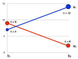
Figure 1. An interaction plot with unequal sample sizes.
First, let's consider the hypothesis for the main effect of B tested by the Type III sums of squares. Type III sums of squares weight the means equally and, for these data, the marginal means for  and
and  are equal:
For /2 = (7 + 9)/2 = 8") .
.
For /2 = (14 + 2)/2 = 8") .
.
Thus, there is no main effect of B when tested using Type III sums of squares. For Type II sums of squares, the means are weighted by sample size.
For /12 = (4 \times 7 + 8 \times 9)/12 = 8.33")
For /20 = (12 \times 14 + 8 \times 2)/20 = 9.2")
Since the weighted marginal mean for is larger than the weighted marginal mean for , there is a main effect of B when tested using Type II sums of squares.
The Type II and Type III analyses are testing different hypotheses. First, let's consider the case in which the differences in sample sizes arise because in the sampling of intact groups, the sample cell sizes reflect the population cell sizes (at least approximately). In this case, it makes sense to weight some means more than others and conclude that there is a main effect of B. This is the result obtained with Type II sums of squares. However, if the sample size differences arose from random assignment, and there just happened to be more observations in some cells than others, then one would want to estimate what the main effects would have been with equal sample sizes and, therefore, weight the means equally. With the means weighted equally, there is no main effect of B, the result obtained with Type III sums of squares.
Unweighted Means Analysis
Type III sums of squares are tests of differences in unweighted means. However, there is an alternative method to testing the same hypotheses tested using Type III sums of squares. This method, unweighted means analysis, is computationally simpler than the standard method but is an approximate test rather than an exact test. It is, however, a very good approximation in all but extreme cases. Moreover, it is exactly the same as the traditional test for effects with one degree of freedom. The Analysis Lab uses unweighted means analysis and therefore may not match the results of other computer programs exactly when there is unequal and the are greater than one.
Causes of Unequal Sample Sizes
None of the methods for dealing with unequal sample sizes are valid if the experimental treatment is the source of the unequal sample sizes. Imagine an experiment seeking to determine whether publicly performing an embarrassing act would affect one's anxiety about public speaking. In this imaginary experiment, the experimental group is asked to reveal to a group of people the most embarrassing thing they have ever done. The control group is asked to describe what they had at their last meal. Twenty subjects are recruited for the experiment and randomly divided into two equal groups of 10, one for the experimental treatment and one for the control. Following their descriptions, subjects are given an attitude survey concerning public speaking. This seems like a valid experimental design. However, of the 10 subjects in the experimental group, four withdrew from the experiment because they did not wish to publicly describe an embarrassing situation. None of the subjects in the control group withdrew. Even if the data analysis were to show a significant effect, it would not be valid to conclude that the treatment had an effect because a likely alternative explanation cannot be ruled out; namely, subjects who were willing to describe an embarrassing situation differed from those who were not. Thus, the differential dropout rate destroyed the random assignment of subjects to conditions, a critical feature of the experimental design. No amount of statistical adjustment can compensate for this flaw.
Video
Questions
Question 1 out of 3.
The biggest problem caused by unequal sample sizes is
- The calculations are extremely difficult.
- The statistical results are only approximate.
- Unequal sample sizes result in confounding.
- Unequal sample sizes indicate a poor experimental design.
Question 2 out of 3.
Which of the following eliminates confounding?
- Unweighted means
- Weighted means
- Correction for continuity
3 out of 3.
Which of the following eliminates confounding?
- Type I sums of squares
- Type III sums of squares
Answers
-
Unequal sample sizes cause confounding.
-
Comparing unweighted means eliminates confounding.
-
Type III sums of squares test an effect while controlling for other effects, thus eliminating confounding.
Tests Supplementing ANOVA
The null hypothesis tested in  one-factor ANOVA is that all the population means are equal. Stated more formally,

where  is the null hypothesis and is the number of conditions. When the null hypothesis is rejected, all that can be said is that at least one population mean is different from at least one other population mean. The methods for doing more specific tests described All Pairwise Comparisons among Means and in Specific Comparisons apply here. Keep in
  nd that these tests are valid whether or not they are preceded by an ANOVA.
Main Effects
As shown below, significant main effects in multi-factor designs can be followed up in the same way as significant effects in one-way designs. Table 1 shows the data from an imaginary experiment with three levels of Factor and two levels of Factor B.
Table 1. Made-Up Example Data.
| A1 | A2 | A3 | Marginal Means | |
|---|---|---|---|---|
| B1 | 5 | 9 | 7 | 7.08 |
| 4 | 8 | 9 | ||
| 6 | 7 | 9 | ||
| 5 | 8 | 8 | ||
| Mean = 5 | Mean = 8 | Mean = 8.25 | ||
| B2 | 4 | 8 | 8 | 6.50 |
| 3 | 6 | 9 | ||
| 6 | 8 | 7 | ||
| 8 | 5 | 6 | ||
| Mean = 5.25 | Mean = 6.75 | Mean = 7.50 | ||
| Marginal Means | 5.125 | 7.375 | 7.875 | 6.79 |
Table 2 shows the ANOVA Summary Table for these data. The significant main effect of indicates that, in the population, at least one of the marginal means for is different from at least one of the others.
Table 2. ANOVA Summary Table for Made-Up Example Data.
| Source | df | SSQ | MS | F | p |
|---|---|---|---|---|---|
| A | 2 | 34.333 | 17.167 | 9.29 | 0.0017 |
| B | 1 | 2.042 | 2.042 | 1.10 | 0.3070 |
|
x B
|
2 | 2.333 | 1.167 | 0.63 | 0.5431 |
| Error | 18 | 33.250 | 1.847 | ||
| Total | 23 | 71.958 |
The Tukey HSD test can be used to test all pairwise comparisons among means in one-factor ANOVA as well as comparisons among marginal means in multi-factor ANOVA. The formula for the equal-sample-size case is shown below.

where and  are marginal means, is the mean square error from the ANOVA, and n is the number of scores each mean is based upon. For this example,
  and
and  because there are eight scores at each level of . The probability value can be computed using the Studentized Range Calculator. The degrees of freedom is equal to the degrees of freedom error. For this example,
  . The results of the Tukey HSD test are shown in Table 3. The mean for
  is significantly lower than the mean for
  and the mean for
  . The means for and are not significantly different.
Table 3. Pairwise Comparisons Among Marginal Means for .
| Comparison | Mi - Mj | Q | p |
|---|---|---|---|
| A1 - A2 | -2.25 | -4.68 | 0.010 |
| A1 - A3 | -2.75 | -5.72 | 0.002 |
| A2 - A3 | -0.50 | -1.04 | 0.746 |
Specific comparisons among means are also carried out much the same way as shown in the relevant section on testing means. The formula for L is
where ci is the coefficient for the ith marginal mean and is the ith marginal mean. For example, to compare with the average of and , the coefficients would be 1, -0.5, -0.5. Therefore,

(5.125) + (-0.5)(7.375) + (-0.5)(7.875) = -2.5") .
.To compute t, use:


where is the mean square error from the ANOVA and n is the number of scores each marginal mean is based on (eight in this example). The degrees of freedom is the degrees of freedom error from the ANOVA and is equal to 18. Using the Online Calculator, we find that the two-tailed probability value is 0.0005. Therefore, the difference between and the average of and is significant.
Important issues concerning multiple comparisons and orthogonal comparisons are discussed in the Specific Comparisons section in the Testing Means chapter.
Interactions
The presence of significant interaction makes the interpretation of the results more complicated. Since an interaction means that the simple effects are different, the main effect as the mean of the simple effects does not tell the whole story. This section discusses how to describe interactions, proper and improper uses of simple effects tests, and how to test components of interactions.
Describing Interactions
A crucial first step in understanding significant interaction is constructing an interaction plot. Figure 1 shows an interaction plot from data presented in the section on Multi-Factor ANOVA.
Figure 1. Interaction Plot for Made-Up Data.
The second step is to describe the interaction in clear and understandable way. This is often done by describing how the simple effects differed. Since this should be done using as little jargon as possible, the expression "simple effect" need not appear in the description. An example is as follows:
The effect of Outcome differed depending on the subject's self-esteem. The difference between the attribution to self following success and the attribution to self following failure was larger for high-self-esteem subjects (mean difference = 2.50) than for low-self-esteem subjects (mean difference = -2.33).
No further analyses are helpful in understanding the interaction since the interaction means only that the simple effects differ. The interaction's significance indicates that the simple effects differ from each other, but provides no information about whether they differ from zero.
Simple Effect Tests
It is not necessary to know whether the simple effects differ from zero in order to understand an interaction because the question of whether simple effects differ from zero has nothing to do with interaction except that if they are both zero there is no interaction. It is not uncommon to see research articles in which the authors report that they analyzed simple effects in order to explain the interaction. However, this is not valid approach since an interaction does not depend on the analysis of the simple effects.
However, there is reason to test simple effects following significant interaction. Since an interaction indicates that simple effects differ, it means that the main effects are not general. In the made-up example, the main effect of Outcome is not very informative, and the effect of outcome should be considered separately for high- and low-self-esteem subjects.
As will be seen, the simple effects of Outcome are significant and in opposite directions: Success significantly increases attribution to self for high-self-esteem subjects and significantly lowers attribution to self for low-self-esteem subjects. This is very easy result to interpret.
What would the interpretation have been if neither simple effect had been significant? On the surface, this seems impossible: How can the simple effects both be zero if they differ from each other significantly as tested by the interaction? The answer is that non-significant simple effect does not mean that the simple effect is zero: the null hypothesis should not be accepted just because it is not rejected.
If neither simple effect is significant, the conclusion should be that the simple effects differ, and that at least one of them is not zero. However, no conclusion should be drawn about which simple effect(s) is/are not zero.
Another error that can be made by stakenly accepting the null hypothesis is to conclude that two simple effects are different because one is significant and the other is not. Consider the results of an imaginary experiment in which the researcher hypothesized that addicted people would show larger increase in brain activity following some treatment than would non-addicted people. In other words, the researcher hypothesized that addiction status and treatment would interact. The results shown in Figure 2 are very much in line with the hypothesis. However, the test of the interaction resulted in probability value of 0.08, value not quite low enough to be significant at the conventional 0.05 level. The proper conclusion is that the experiment supports the researcher's hypothesis, but not strongly enough to allow confident conclusion.
Figure 2. Made-up Data with One Significant Simple Effect.
Unfortunately, the researcher was not satisfied with such weak conclusion and went on to test the simple effects. It turned out that the effect of Treatment was significant for the Addicted group ") but not significant for the Non-Addicted group
but not significant for the Non-Addicted group ") . The researcher then went on to conclude that since there is an effect of Treatment for the Addicted group but not for the Non-Addicted group, the hypothesis of greater effect for the former than for the latter group is demonstrated. This is faulty logic, however, since it is based on accepting the null hypothesis that the simple effect of Treatment is zero for the Non-Addicted group just because it is not significant.
. The researcher then went on to conclude that since there is an effect of Treatment for the Addicted group but not for the Non-Addicted group, the hypothesis of greater effect for the former than for the latter group is demonstrated. This is faulty logic, however, since it is based on accepting the null hypothesis that the simple effect of Treatment is zero for the Non-Addicted group just because it is not significant.
Components of Interaction (optional)
Figure 3 shows the results of an imaginary experiment on diet and weight loss. control group and two diets were used for both overweight teens and overweight adults.
Figure 3. Made-up Data for Diet Study.
The difference between Diet and the Control diet was essentially the same for teens and adults, whereas the difference between Diet B and Diet was much larger for the teens than it was for the adults. Over one portion of the graph the lines are parallel whereas over another portion they are not. It is possible to test these portions or components of interactions using the method of specific comparisons discussed previously. The test of the difference between Teens and Adults on the difference between Diets and B could be tested with the coefficients shown in Table 4. Naturally, the same considerations regarding multiple comparisons and orthogonal comparisons that apply to other comparisons among means also apply to comparisons involving components of interactions.
Table 4. Coefficients for Component of the Interaction.
| Age Group | Diet | Coefficient |
|---|---|---|
| Teen | Control | 0 |
| Teen | A | 1 |
| Teen | B | -1 |
| Adult | Control | 0 |
| Adult | A | -1 |
| Adult | B | 1 |
Video
Questions
Question 1 out of 7.
When the null hypothesis is rejected in ANOVA, the ANOVA test reveals which means are significantly different from which other means.
- True
- False
Question 2 out of 7.
A marginal mean is
- A mean that is almost significant.
- The mean of the means of one variable averaging over the levels of another variable.
Question 3 out of 7.
A main effect is a comparison of
- Marginal means
- Standardized means
- Simple effects
Question 4 out of 7.
To compare a control group with the average of the other three groups, you would use
- Tukey's test
- An interaction test
- A specific comparison
Question 5 out of 7.
To compare each mean with each other mean, you would use
- Tukey's test
- An interaction test
- A specific comparison
- ANOVA
Question 6 out of 7.
An interaction makes it difficult to interpret
- simple effects
- pairwise comparisons
- specific comparisons
- main effects
Question 7 out of 7.
If one simple effect is significant and another is not, that means there is an interaction.
- True
- False
Answers
-
Rejecting the null hypothesis only indicates that at least one population mean is different from at least one other.
-
The mean of the means of one variable averaging over the levels of another variable.
-
Marginal means
-
A specific comparison
-
Tukey's test
-
Main effects. The interaction means the simple effects differ and therefore the main effect does not tell the whole story.
-
False, because it is not valid to accept the null hypothesis that a simple effect is 0 when it is not significant.
Power of Within-Subjects Designs Demonstration
Instructions
This simulation demonstrates the effect of the correlation between measures in a one-way within-subjects ANOVA with two levels. This test is equivalent to a correlated t test. The default values for this demonstration are for an experiment with 10 subjects each measured under two conditions. The population difference for the two conditions is 1.85 and the variance in each of the conditions is 4.0. The graph shows the power of the test as a function ofthe population correlation between the two scores for the 0.10, 0.05, and 0.01 significance levels. The power of an independent-groups t test (which assumes the correlation is 0) is shown by the x's.
Experiment with different combinations of the parameters. Is the correlation an important factor in power?
Illustrated Instructions
The video begins by changing the population variance to 8 and increases the sample size to 25 and then reduces it to 5. Notice the impact that these changes have on the relationship between power and population correlation. The video concludes by changing the mean difference to 4.
Questions
Question 1 out of 4.
Increasing the correlation between measures:
- increases power.
- decreases power.
- has no effect on power.
Question 2 out of 4.
Increasing the population variance:
- increases power.
- decreases power.
- has no effect on power.
Question 3 out of 4.
Increasing the difference between population means:
- increases power.
- decreases power.
- has no effect on power.
Question 4 out of 4.
Assuming the hypothesized direction of the effect is correct, a one-tailed test is:
- more powerful than a two-tailed test.
- less powerful than a two-tailed test.
- has the same power as a two-tailed test.
Answers
-
High correlations can result in much higher power than lower correlations. They do this by lowering the mean square error.
-
High variance increases the error term and lowers power.
-
The more different the population means, the bigger the effect and the higher the power.
-
Since the probability is caluclated in only one tail, a one-tailed test results in a lower probability value.
Statistical Literacy
Testing an Alzheimer's Drug
A research design to compare three drugs for the treatment of Alzheimer's disease is described here. For the first two years of the study, researchers will follow the subjects with scans and memory tests.
What do you think?
Assume the data were analyzed as a two-factor design with pre-post testing as one factor and the three drugs as the second factor. What term in an ANOVA would reflect whether the pre-post change was different for the three drugs?
It would be the interaction of the two factors since the question is whether the effect of one factor (pre-post) differs as a function of the level of a second factor (drug).
Weight Loss and Cancer Risk
An experiment on risk factors for cancer had four conditions related to weight loss. Quoting the web page description:
"McTiernan and her colleagues randomly assigned 399 overweight and obese postmenopausal women to one of four groups - dieting plus exercise, dieting only, exercise only or a control group not required to do either".
What do you think?
There are two between-subjects factors: Diet (yes or no) and Exercise (yes or no) resulting in the four conditions. The design is a 2 x 2 factorial design.
Exercises
-
What is the null hypothesis tested by analysis of variance?
-
What are the assumptions of between-subjects analysis of variance?
-
What is a between-subjects variable?
-
Why not just compute t-tests among all pairs of means instead computing an analysis of variance?
-
What is the difference between "N" and "n"?
-
How is it that estimates of variance can be used to test a hypothesis about means?
-
Explain why the variance of the sample means has to be multiplied by "n" in the computation of MSB.
-
What kind of skew does the F distribution have?
-
When do MSB and MSE estimate the same quantity?
-
If an experiment is conducted with 6 conditions and 5 subjects in each condition, what are dfn and dfe?
-
How is the shape of the F distribution affected by the degrees of freedom?
-
What are the two components of the total sum of squares in a one-factor between-subjects design?
-
How is the mean square computed from the sum of squares?
-
An experimenter is interested in the effects of two independent variables on self esteem. What is better about conducting a factorial experiment than conducting two separate experiements, one for each independent variable?
-
An experiment is conducted on the effect of age and treatment condition (experimental versus control) on reading speed. Which statistical term (main effect, simple effect, interaction, specific comparison) applies to each of the descriptions of effects.
- The effect of the treatment was larger for 15-year olds than it was for 5- or 10-year olds.
- Overall, subjects in the treatment condition performed faster than subjects in the control condition.
- The difference between the 10- and 15-year olds was significant under the treatment condition.
- The difference between the 15- year olds and the average of the 5- and 10-year olds was significant.
-
As they grow older, children read faster.
-
An A(3) x B(4) factorial design with 6 subjects in each group is analyzed. Give the source and degrees of freedom columns of the analysis of variance summary table.
-
The following data are from a hypothetical study on the effects of age and time on scores on a test of reading comprehension. Compute the analysis of variance summary table.
-
Define "Three-way interaction"
-
Define interaction in terms of simple effects.
-
Plot an interaction for an A(2) x B(2) design in which the effect of B is greater at A1 than it is at A2. The dependent variable is "Number correct." Make sure to label both axes.
- Following are two graphs of population means for 2 x 3 designs.
For each graph, indicate which effect(s) (A, B, or A x B) are
nonzero.
-
The following data are from an A(2) x B(4) factorial design.
- Compute an analysis of variance.
- Test differences among the four levels of B using the Bonferroni correction.
- Test the linear component of trend for the effect of B.
- Plot the interaction.
-
Describe the interaction in words.
- Why are within-subjects designs usually more powerful than
between-subjects design?
- What source of variation is found in an ANOVA summary table
for a within-subjects design that is not in in an ANOVA summary
table for a between-subjects design. What happens to this source
of variation in a between-subjects design?
-
The following data contain three scores from each of five subjects. The three scores per subject are their scores on three trials of a memory task.
4 6 7
3 7 7
2 8 5
1 4 7
4 6 9- Compute an ANOVA
- Test all pairwise differences between means using the Bonferroni test at the .01 level.
-
Test the linear and quadratic components of trend for these data.
-
Give the source and df columns of the ANOVA summary table for the following experiments:
- Twenty two subjects are each tested on a simple reaction time task and on a choice reaction time task.
- Twelve male and 12 female
subjects are each tested under three levels
of drug dosage: 0 mg, 10 mg, and 20 mg. - Twenty subjects are tested on a motor learning task for three trials a day for two days.
- An experiment is conducted in which
depressed people are either assigned to a drug therapy
group, a behavioral therapy group, or a control group.
Ten subjects are assigned to each group. The level of measured
once a month for four months.
| 12-year olds | 16-year olds | |
| 30 minutes | 66 68 59 72 46 |
74 71 67 82 76 |
| 60 minutes | 69 61 69 73 61 |
95 92 95 98 94 |
| B1 | B2 | B3 | B4 | |
| A1 | 1 3 4 5 |
2 2 4 5 |
3 4 2 6 |
4 |
| A2 | 1 1 2 2 |
2 3 2 4 |
4 6 7 8 |
8 9 9 8 |
Questions from Case Studies:
The following question is from the Stroop Interference case study.
-
The dataset has the scores (times) for males and females on each of three tasks.
a. Do a Gender (2) x Task (3) analysis of variance.
b. Plot the interaction.
The following question is from the ADHD Treatment case study.
-
The data has four scores per subject.
- Is the design between-subjects or within-subjects?
- Create an ANOVA summary table.
The following question is from the Angry
Moods case
study.
-
Using the Anger Expression Index as the dependent variable, perform a 2x2 ANOVA with gender and sports participation as the two factors. Do athletes and non-athletes differ significantly in how much anger they express? Do the genders differ significantly in Anger Expression Index? Is the effect of sports participation significantly different for the two genders?
The following question is from the Weapons
and Aggression case
study. - Compute a 2x2 ANOVA on this data with the following
two factors: prime type (was the first word a weapon or not?)
and word type (was the second word aggressive or non-aggressive?). Consider
carefully whether the variables are between-subject or within-subects
variables.
The following question is from the Smiles
and Leniency case
study. - Compute the ANOVA summary table.