MA121 Study Guide
| Site: | Saylor University |
| Course: | MA121: Introduction to Statistics |
| Book: | MA121 Study Guide |
| Printed by: | Guest user |
| Date: | Sunday, 21 June 2026, 8:31 AM |
Description
Navigating the Study Guide
Study Guide Structure
In this study guide, the sections in each unit (1a., 1b., etc.) are the learning outcomes of that unit.
Beneath each learning outcome are:
- questions for you to answer independently;
- a brief summary of the learning outcome topic;
- and resources related to the learning outcome.
At the end of each unit, there is also a list of suggested vocabulary words.
How to Use the Study Guide
- Review the entire course by reading the learning outcome summaries and suggested resources.
- Test your understanding of the course information by answering questions related to each unit learning outcome and defining and memorizing the vocabulary words at the end of each unit.
By clicking on the gear button on the top right of the screen, you can print the study guide. Then you can make notes, highlight, and underline as you work.
Through reviewing and completing the study guide, you should gain a deeper understanding of each learning outcome in the course and be better prepared for the final exam!
Unit 1: Statistics and Data
1a. Describe types of sampling methods for data collection
- What is the difference between a population and a sample?
- What is the definition of bias and inferential data?
- How can researchers control for possible bias in samples?
- What is the definition of a sample and sample size?
- What are the definitions of the three types of sampling: stratified, cluster, and systematic?
A population is everyone we would like to collect data about. For example, if we study the voting habits of 20- to 25-year-olds in the US, we see that the population would be every 20- to 25-year-old in the US. However, it is not always practical or even possible to collect data from every single person we are trying to study, so we collect a sample. A sample is a subset of the population we use to draw conclusions about the entire population. A sample size is the number of data points or people in your sample.
Bias (systematic error that causes results to consistently deviate from the true value or misrepresent the population being studied) occurs when we deal with inferential statistics. For example, because we cannot practically consider every person in the United States as part of our dataset, we have to ensure our sample represents the entire population.
A common example of how things can go wrong is the 1936 US presidential election, when political polling was brand new. The Literary Digest magazine mailed thousands of survey cards to its readers and people, which it found in the phone book and car registration directory, to poll whether Republican challenger Alf Landon would defeat the Democratic incumbent Franklin D. Roosevelt. The responses predicted Landon would win in a landslide. What went wrong?
Their sample size was large enough, and their mathematical calculations were probably correct. However, in 1936, phones, cars, and even magazine subscriptions were considered luxury items. The magazine's sample disproportionately represented wealthier Americans who were more likely to vote Republican.
While it is difficult to eliminate sampling bias entirely, we can use different sampling methods to reduce it.
- Stratified sampling divides the population into sub-populations and takes a random sample of each group. For example, if you think Democrats, Republicans, and Independents will poll differently on an issue, and these groups each represent 30, 25, and 45 percent of the entire US population, your sample should reflect the same proportion of representatives. You should choose 30 Democrats, 25 Republicans, and 45 independents at random and send the survey form to all of these 100 individuals.
- Researchers use cluster sampling when their population is already divided into representative groups. For example, a researcher might study buildings (or clusters) in an apartment complex, choose a certain number of buildings at random, and sample everyone in each building.
- Researchers use systematic sampling when they have a rough idea of population size but lack a representative cluster to sample. For example, a researcher might poll every tenth person who walks through the door in a shopping mall, or an inspector might examine every 20th item on an assembly line for quality.
Review
To review, see:
1b. Interpret frequency tables
- What is a frequency table?
- What are the definitions of class, bin, and class intervals?
- What is the definition of an outlier?
- Why is it important to include every possible value between the lowest and highest on the left side of a frequency table, even when that value is not represented or has no frequency? In other words, if the data you obtain from an experiment ranges from 1 to 5 and there are no 4s, why do you need to display a row for 4?
- What do you do when there are too many values in a data set to give each variable its own row? Let's say the variable is yards rushing during a football game, and the possible values are 51 to 218. Your space does not allow you to display more than 160 rows in your table. What do you do?
A frequency table lists every possible value of the random variable (every possible value) in a data distribution. It must include an interior value, even when that data point has no frequency. This is because one of the purposes of a frequency table is to display how varied the data is.
For example, if our values are 1, 2, 3, and 25, you should space the 25 so it is 22 points away from the three to illustrate how much of an outlier it is. You should include rows for 4 to 24, with a zero frequency for each.
If the distribution has too many possible values, you can group the values into class intervals (sometimes called classes or bins) and mark the frequency for each.
Let's return to our football example. You can display the number of players who have rushed 50 to 59 yards, 60 to 69 yards, and so on. If you treat this data as discrete, it will be a long, tedious table with mostly ones and zeros since you would need to show the number of players who rushed 50 yards, the number of players who rushed 51 yards, the number of players who rushed 52 yards, and so on. Grouping or organizing the figures into classes of ten yards each is more concise and gives the reader a more comprehensive picture of the total data.
If you group your data into classes, make sure:
- Each class is the same width,
- Each class does not overlap, and
- Each class accounts for every possible value.
For example, we could use 50 to 59 yards, 60 to 69 yards, and so on. Each class width would equal ten rushing yards. We should not use 50 to 55 yards, 56 to 70 yards, or 71 to 73 yards.
Note that we are assuming the measurements are in whole yards. If we had a measurement of 55.3 in the above grouping, we would violate our third rule (that each class accounts for every possible value) since 55.3 comes between two classes. So you may have to group your data as 50 to 55, 55 to 60, and so on, so you would put 55.5 and even 55.99 in the first class or bin.
Your decision on how wide to make your class interval and how many intervals to include is a matter of personal preference. The course refers to formulas like Sturges' Rule and Rice Rule, which are easy to compute (the number of intervals equals the cube root of the number of observations). However, you may need to make some adjustments since your result will probably not be a whole number (integer).
Do not worry too much about memorizing these rules since statisticians do not even agree on which rule is best. Researchers generally recommend using 5 to 20 class widths, but this can vary depending on whether your data is homogenous or heterogenous. It might be a good strategy to put your data in groups of tens so you can classify each data point by its first digit.
If you have too few classes, your readers may not appreciate the diversity of your data. If you have too many classes, you will probably display many ones and zeros, which can become tedious for the reader. Experiment with a few options until you see one that makes sense to you and your audience.
Review
To review, see:
1c. Display data graphically in stem plots, histograms, boxplots, and scatterplots
- What is the definition of a histogram? How does it differ from a bar graph? What are some rules for drawing histograms that do not apply to bar graphs?
- How is a stem plot similar to and different from a histogram?
- What is a dot plot?
- What does a boxplot represent graphically?
- What is a scatterplot, and how is it different from the other three graphs discussed here?
A histogram is a special type of bar graph that researchers use to display quantitative distributions. A histogram differs from a bar graph because the horizontal axis is numeric: the horizontal axis of a bar graph represents qualitative data, and the vertical axis represents the frequency.
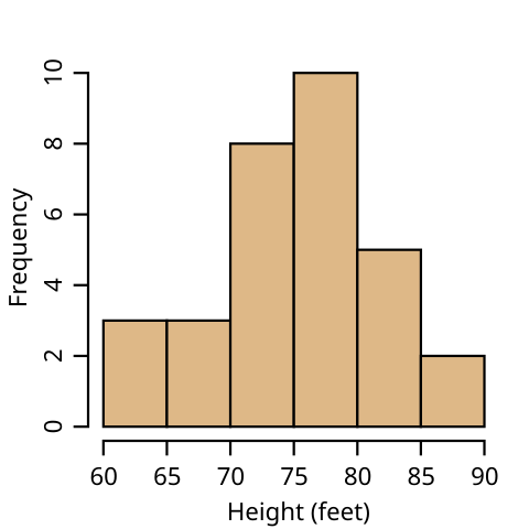
A histogram should follow the same three rules for frequency tables listed above. The numbers on the horizontal axis need to be in order if they are grouped into classes. This makes it easy for readers to recognize any data point that is an outlier (a data value that is significantly different from the other values in the dataset) due to the distance of the outlier's bar from the other bars in the graph. You must include any data point or interval that has zero values with no bar. For consistency, data that is homogenous (or heterogenous) is organized in the same way on the histogram. Remember that a histogram's main purpose is to represent a frequency table graphically.
A stem plot (also called a stem-and-leaf plot) is similar to a histogram, except it includes the last digit of the actual data values (the leaves) above the stem of the first digit or digits. Researchers use a stem plot to display the actual data on their graph. Stem plots quickly convey the minimum, maximum, and median of the data points to their readers.
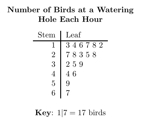
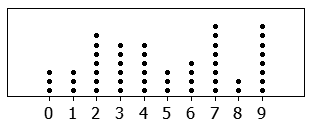
A stem plot is similar to a dot plot, which uses dots or similar markings to represent data points. For example, if the bar height (frequency) of the histogram is seven, and the values are 50, 51, 52, 54, 55, 56, and 59, the histogram will display a bar that is seven units high. A dot plot will have seven dots going up from the horizontal axis, and a stem plot will have "five" in the stem, with the digits 1, 2, 4, 5, 6, and 9 written out to the right.
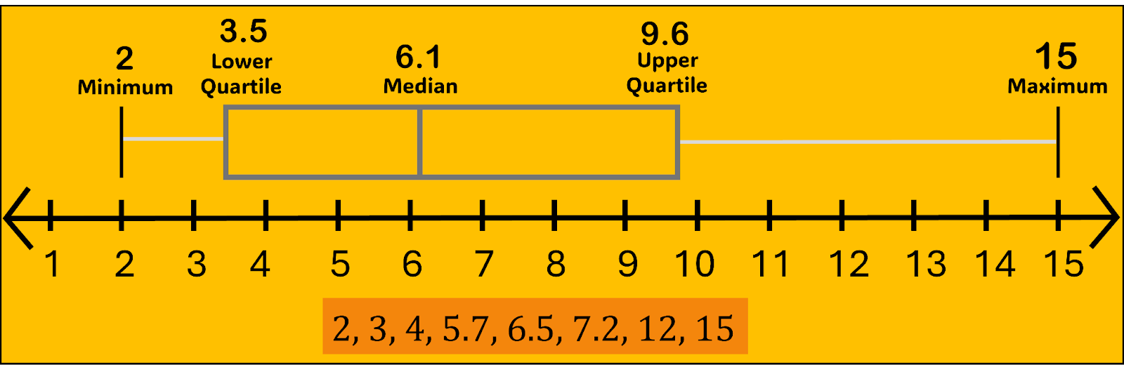
A box plot graphically displays the five-number summary of a data set. The five numbers are the minimum, first quartile, median, third quartile, and maximum. Think of the first and third quartiles as the median of the lower and upper halves of the distribution, respectively. In other words, the five numbers partition the data set into four quartiles, each with (roughly) the same number of data points.
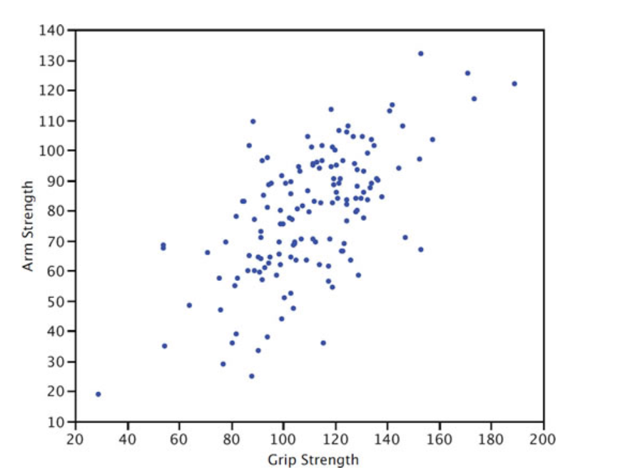
A scatterplot is a graph that shows the relationship between two variables. The scatterplot below shows the arm strength compared to grip strength. Each dot represents one person.
Review
To review, see:
1d. Calculate measures of the location of data: quartiles and percentiles
- What is a percentile, and how is it related to or different from a quartile?
- What is the relationship between quartiles and the median?
- What is the five-number summary?
- A calculator and Excel might give two numbers for the 1st and 3rd quartiles. Why is that?
The Pth percentile of a data set means that P% of the data falls below that number and (100−P)% falls above that number. For example, the 80th percentile is the number where 80% of the data is below and 20% is above. The median (half the data below, half above) is also the 50th percentile. These are approximate, especially for small data sets. This is because, for example, if you have 20 data points, finding the 37th percentile will not be an exact number. Since there are only 20 numbers (assuming no repeats), you'll have a 35th percentile; the next number will be the 40th.
The quartiles of a data set divide that data set into four roughly equally sized (number of data points) parts. Again, we say "roughly" because if the number of data points is small and not a multiple of 4 (17 data points, for example), you will not get four quartiles of the same size. This is another reason why finding quartiles is approximate.
When you have large data sets (100 or more), you can find theoretical percentiles using the Normal Distribution (see Unit 2). The median is the same thing as the 2nd quartile. The 1st quartile divides the first half of the data in half, and the 3rd quartile splits the upper half of the data. The minimum, 1st quartile, median/2nd quartile, 3rd quartile, and maximum make up the boundaries of the four quarters of data and are referred to as the five-number summary.
Finding quartiles for small data sets can be tricky and even subjective if the number of data points is not a multiple of four. In the set: {0, 3, 4, 6, 8, 11, 11, 13, 15, 17, 20, 25}, the median is 11, the first quartile (separating the 3rd and 4th point) is 5, and the third quartile (separating the 9th and 10th point) is 16. This is relatively simple because we have 12 data points and can evenly divide them into groups of 3: {0, 3, 4 || 6, 8, 11 || 11, 13, 15 || 17, 20, 25}.
However, let's say we have 15 data points: {1, 3, 4, 5, 7, 8, 10, 10, 11, 13, 15, 16, 19, 20, 25}. The 2Q/median is the 8th data point (10). What about the 1st quartile? If we include the median, the first half is {1, 3, 4, 5, 7, 8, 10, 10}, and the 1st quartile (the median of this set) is 6. If we exclude the median {1, 3, 4, 5, 7, 8, 10}, then the 1st quartile is 5. That is why different technologies may give you different answers. Which is correct? Well, both. Even Microsoft Excel has two different functions for quartiles: inclusive and exclusive. This discrepancy disappears as the data set gets very large.
Review
To review, see:
1e. Calculate measures of the center of data: mean, median, and mode
- What are the differences between the mean and the median?
- What does the center of distribution tell us?
- When is the median a better measure of center than the mean?
- When is the mode preferable to the mean or median?
We calculate the mean by adding all the data points and dividing the result by the size. The mean provides a rough idea of the center of the distribution. The median does this, too, but disregards all data points except for the one or ones in the middle.
You can think of the median (the middle value in a dataset when all values are arranged in order from lowest to highest) as more resistant to outliers. In other words, when a researcher adds a significantly higher or lower value to a data set, or if the data is right or left-skewed, the mean will adjust accordingly, with a significant upward or downward effect. To be skewed means the data distribution is asymmetrical, with values concentrated more on one side and a tail extending toward the other. Conversely, the median disregards the high and low values, so adding extreme values will have a much smaller (if any) effect on the median.
The mode conveys the most common data type. It differs from the mean and median because it is the only measure of center we can use with qualitative data since it does not require a calculation or computation.
Review
To review, see:
1f. Calculate measures of the spread of data: variance, standard deviation, and range
- Why is range generally not a reliable measure of spread?
- Why are measures of spread necessary? What critical information does the measure of center fail to provide?
- What is the difference between variance and standard deviation?
Measures of spread are just as important as measures of center. The mean and median, for quantitative data, give us an idea about where the center of the distribution is.
The variance and standard deviation tell us about the spread of the data or how varied or heterogeneous your data is. A variance of zero happens if all data points are equal. For example, the data sets {49, 50, 51} and {0, 50, 100} have the same mean and median (50), but the second set is much more varied. We quantify this variability with the measure of spread.
The variance equals the mean of the squared differences between each data point and the mean.
The standard deviation equals the square root of the variance. One of the reasons we compute this is to get the units back to the original data set. If the data points are in minutes, the unit for the variance would be "square minutes", which does not make sense.
The simplest measure to use is the range (maximum to minimum), but the range is generally not a good measure since it only considers the highest and lowest data points.
Consider Data Set A={47,48,49,50,51} and Data Set B={47,48,49,50,51,100}.
The range goes from four to 53. Set B is certainly more varied, but the 100 is an outlier, so the change in standard deviation is less extreme. The standard deviation is 1.6 for set A and 20.9 for set B.
Review
To review, see:
1g. Describe the differences between independent and dependent variables, discrete and continuous variables, and qualitative and quantitative variables
- What is the difference between descriptive and inferential statistics?
- How do quantitative and qualitative data differ?
- What are discrete and continuous data, and how do they differ as types of quantitative data?
- What is the difference between independent and dependent variables?
Descriptive statistics provide facts about a data set, which are often depicted in a graph. Where is the data centered? What is the mean? What is the median? Are the data centered or bell-shaped, meaning they form a symmetrical curve where most values cluster around the center and taper off equally on both sides? Is the distribution curved, showing a peak and then gradually decreasing, but not necessarily in a symmetrical way? Are the data skewed to the right or left? In other words, do most values appear at one end of the graph? These descriptions tell us facts about the data in front of us and our chosen population or sample.
Inferential statistics refers to how we draw conclusions about a population of data when we examine data in a sample. Inferential statistics is the more common method of statistics since we rarely have the time or resources to survey or measure every item, member, or person in a given group or population. In statistics, differences among various data types are important since they determine which tests or graphs are most useful for displaying data and answering certain questions.
Quantitative data (or numeric data) describes numeric or mathematical data. We use quantitative data to calculate sums, averages, means, other types of statistics, and other mathematical operations.
Qualitative data (or categorical data) describes non-numeric data. Qualitative data includes text, letters, and words. Qualitative data can also include numerical digits, but mathematical operations do not make sense or may be impossible in this usage.
For example, consider a phone number, zip code, or postal code. Although these designations consist of numerical digits (numbers) and may include dashes and parentheses, we do not use them to conduct calculations. We do not add or calculate an average for the numbers in our telephone contact list or postal code. Phone numbers, zip codes, and postal codes are examples of qualitative data.
We can categorize quantitative data further as discrete or continuous data.
A discrete data set contains a fixed or small number of possible values. The classic example of a discrete data set is a six-sided die. You can only roll a one, two, three, four, five, or six. You cannot roll a 2.8.
A continuous data set has a large or infinite number of possibilities. Consider the weight of a group of college students. When we discard extreme outliers, our range may be from 120 to 200 pounds. This dataset includes 61 possible values, assuming we measure while rounding to the nearest pound. When a 285-pound football player enters our dataset, we must add 85 possibilities to account for 166 possible values because the dataset is continuous. Although this number is not infinite, it is impractical to consider it as discrete data, as we will review in the next learning outcome.
Independent variables are the variables researchers manipulate to see if they affect the dependent variable. For example, if we are studying a new diet pill for weight loss, we could give half of the rats in our study a new one. Then, we would record any weight change in the two groups of rats. The diet pill would be the independent variable, while the weight change would be the dependent variable.
Review
To review, see:
1h. Explain what information Pearson's correlation coefficient gives about the dataset
- What does Pearson's correlation coefficient measure?
- What are the possible values for Pearson's coefficient?
Pearson's correlation coefficient measures the strength of the linear relationship between two variables. This coefficient can range from -1 to 1. A -1 would represent a perfect negative relationship between the two variables, while a coefficient of 1 would represent a perfect positive relationship. Consider the number of hours someone spends running and their cardio fitness. We would expect this to be a positive relationship. At the same time, we would expect that more hours watching TV would negatively affect test scores. A correlation of 0 would mean there is no linear relationship between the two variables.
Review
To review, see:
Unit 1 Vocabulary
This vocabulary list includes terms you will need to know to successfully complete the final exam.
- bias
- box plot
- class interval
- cluster sampling
- continuous data
- dependent variable
- descriptive statistics
- discrete data
- dot plot
- frequency table
- histogram
- independent variable
- inferential statistics
- mean
- median
- mode
- outlier
- Pearson's correlation coefficient
- population
- qualitative data
- quantitative data
- quartile
- range
- sample
- sample size
- scatterplot
- skewed
- standard deviation
- stem plot
- stratified sampling
- systematic sampling
- variance
Unit 2: Elements of Probability and Random Variables
2a. Calculate conditional probability
- What is the definition of probability, and how is probability computed?
- What does the concept of equally likely outcomes mean?
- What is a random variable, and how does it differ from variables used in Algebra?
- What are the types of random variables?
Think about probability as the chance that an outcome or event will occur. The probability of something occurring is a number between 0 (zero percent or no chance) and 1 (100 percent or definitely).
We always express probability as a decimal for use in calculations. In other words, we write 55 percent as p=0.55. If you have several events with equally likely outcomes, then the number of possible outcomes is the denominator, and the number of "successful" outcomes is the numerator.
For example, the probability of rolling greater than four on a six-sided die is 2/6 because rolling a five and a six are the successes out of six outcomes. We cannot extend this to the sum of two dice. Totals of 2 through 12 make eleven possible events, but not all of them are equally likely. There is only one way {1,1} to roll a 2, but six ways {1,6}, {2,5}, {3,4}, {4,3}, {5,2}, {6,1} to roll a 7.
There are many variations of the probability formula for different situations and distributions, but we generally calculate probability as the number of "favorable" outcomes (that is, outcomes you are looking for) divided by the total number of possible outcomes.
A random variable differs from variables you have seen in algebra because the value of x is fixed in those courses, and we solve for its value by following certain steps.
For example, for the equation 2x=4, x always equals 2; it is just a matter of finding it. The study of probability introduces the concept of random variables: their value results from a probability experiment.
If x equals the number of times a coin lands on heads when you flip a coin five times, x will have a value from zero to five. We do not know the specific value until we have tossed the coin five times.
A random variable (a function that assigns numerical values to the outcomes of a random process or experiment) can be discrete (only allowing a specific set of possible values) or continuous (many or an infinite number of possible values).
In our coin toss example above, x is a discrete random variable since x can only have six possible values (0 to 5). A continuous random variable might be a team's score during a basketball game. As discussed above, there are too many possible values to make a frequency table for each potential point value.
Review
To review, see:
2b. Calculate probabilities using the addition rules and multiplication rules
- What is the general addition rule of probability, and how does it relate to whether events are mutually exclusive?
- What is the multiplication rule of probability, and how does it relate to whether events are independent?
- What are the special addition, general multiplication, and special multiplication rules in probability?
Compound events are events that consist of two or more simple events combined. We generally associate the general addition rule of probability with "or" compound events. We associate the multiplication rule with "and" compound events.
The probability P(A|B)=P(A)+P(B) holds if A and B are mutually exclusive (cannot both occur).
If A and B are not mutually exclusive, the special addition rule holds: P(A|B)=P(A)+P(B)-P(A&B).
The general multiplication rule is P(A&B)=P(A)×P(B) and holds if A and B are independent.
If they are dependent events, that's when conditional probability comes in. Conditional probability is the probability of an event occurring, given that another event has already happened. In this situation, we use the special multiplication rule: P(A&B)=P(A)×P(B|A).
Review
To review, see:
2c. Interpret Venn diagrams
- What is the definition of a union or an intersection of events in probability?
- How can Venn diagrams be used to illustrate outcomes and events?
The probability of a union of events P(A⋃B) is the same as either A or B (or both) happening.
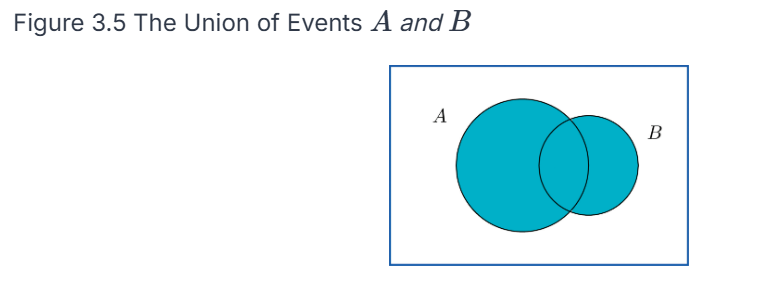
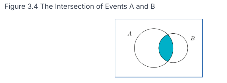
The probability of an intersection of events P(A ⋂ and B) is the same as saying that both A and B happen. We can represent these on a Venn diagram as events (circles) where outcomes are points in each circle. A union would be pictured as both circles shaded in, whereas an intersection would be represented as only the common area being shaded in.
Review
To review, see:
2d. Apply counting rules in the context of combinatorial probability
- What is the definition of a combination, and how is it different from a permutation?
- What are the formulas used to find the number of combinations and the number of permutations?
A combination or permutation refers to the number of possible ways that x out of a possible n outcomes can occur. The difference is that, in a combination, the order does not matter; in a permutation, the order does matter.
For example, there are ten ways to choose x=2 out of the first n=5 letters of the alphabet: AB, AC, AD, AE, BC, BD, BE, CD, CE, and DE. If order does not matter, ten combinations are possible. You could reverse the order of any of the letters, and it would not matter.
There would be 20 permutations if AB and BA were considered different. Without listing them all here, you can intuitively see this because you have ten combinations, and each combination can be in two different orders (AB or BA), so 10×2=20 permutations.
To find the number of ways you can pick r items out of a group of n things, given a permutation, meaning order matters, you use the formula:
!}")
If you are not concerned about the order the items are picked in, you use the formula for combinations:
!\mathrm{r}!}")
Review
To review, see:
2e. Identify common discrete probability distribution functions
- What is a probability distribution, and how does it relate to the frequency tables reviewed in Unit 1?
- What is the difference between a discrete and a continuous probability distribution?
A probability distribution consists of each possible value (or interval of values) of a random variable and the probability that the variable will take on that value.
Probability distributions have many implications in decision-making. When you interpret data, you must know the probability distribution of the value you are trying to estimate. They are related to the frequency tables in that the probabilities are equivalent to the relative frequency distribution.
If you have a list of data, you can get the probabilities on the right side of the table by dividing the frequency by the total number of data points. For example, if the frequency of x=3 is 7 in 20 die rolls, then the probability of rolling a three is 7/20=0.35, so 0.35 would go across from value 3 in the table.
The difference between discrete and continuous probability distributions is analogous to the difference between discrete and continuous variables.
A discrete distribution (like a die roll) has a fixed, finite set of possible values for the random variable x. In contrast, a continuous distribution has many or infinitely many possible values for x. Like a frequency distribution, the values of x must be grouped into intervals. The same rules apply as those that apply to relative frequency histograms: all intervals must be equal in width, non-overlapping, and all-inclusive.
Review
To review, see:
2f. Calculate expected values
- What is the expected value of a distribution, and how is it related to the mean of a set of data?
- What is the formula for expected value?
The expected value of a distribution is another name for the mean of the distribution.
This means that if you take a large set of numbers that follows the original distribution, the arithmetic mean (sum divided by n) of those numbers should roughly equal the expected value of the distribution.
We calculate the value of a distribution by multiplying each value of x by its probability (the median of the interval if it is continuous) and then summing up those numbers.
The formula is ") .
.
This tells us the expected value of x after doing many trials of the experiment.
Review
To review, see:
- Random Variables and Probability Distributions
- Binomial Distributions
- Binomial, Poisson, and Multinomial Distributions
2g. Apply the binomial probability distribution
- What is a binomial experiment?
- What is a binomial distribution?
- What characteristics must a set of events have to follow a binomial distribution?
A binomial experiment is a random experiment that has exactly two possible values (quantitative or qualitative) for x:
- Flipping a coin: x={heads, tails}
- Answer to a true-false question: x={true, false}
- Free throw in basketball: x={made, not made}
A binomial distribution is the distribution of the discrete random variable x, where x represents the number of successes out of n possible events. Note that we mean success in a generic sense: success may not be positive. "Success" means the characteristic you are looking for or researching, regardless of whether you consider the outcome good or bad.
In our basketball free-throw example, if a player takes 10 free-throw shots, they will be successful zero to 10 times. Possible values for x include {0, 1, 2, 3, 4, 5, 6, 7, 8, 9, 10}.
These values and their associated probabilities comprise a binomial probability distribution, which must have three criteria:
- All experiments are binomial.
- All experiments will succeed or fail independently (that is, all free throws are independent events).
- All experiments have an equal probability of success.
A binomial distribution is a family of distributions where each specific distribution consists of two parameters: n is the number of experiments, and p is the probability of success per experiment.
For our basketball example, if the player hits their free throws 75% of the time, we would define this distribution as binomial with n=10 and p=0.75. There are infinite possible binomial distributions, with each combination of n and p making a unique distribution.
Any specific distribution within a family of distributions is defined by its parameters (numerical values determining the particular shape and characteristics of a probability distribution). For example, binomial distributions have parameters n and p. We can calculate the expected value of this distribution by multiplying n and p, or n × p.
Review
To review, see:
2h. Apply the Poisson probability distribution
- What is the definition of a Poisson distribution? When can you use it to estimate a binomial distribution?
- How would you describe a second general use for the Poisson distribution in addition to approximating a binomial distribution?
- A binomial distribution with n=20 and p=0.4 gives the same lambda (or mean) and Poisson distribution as a binomial distribution with n=2000 and p=0.004. How can the same Poisson distribution be "equivalent" to multiple binomial distributions?
The Poisson distribution (pronounced pwah-SOHN or ˈpwɑːsɒn) is related to the binomial distribution because you can use it to approximate the binomial distribution when n is a large value and p is a small value. Unlike the binomial distribution, the Poisson distribution is easier to calculate because it has only one parameter (represented by the Greek letter λ) and the expected value. The calculation is n × p, just as for the binomial distribution.
Statisticians refer to the Poisson distribution as the distribution of rare events. Suppose 1,000 cars drive on a section of road daily, and 1.2 of them get into an accident on average. Since the mean is so small compared to n, we can model this using a Poisson distribution with λ=1.2. We can use the formula to find the probability of x=1 accident, x=2 accidents, and so on.
A minor difference between the Poisson distribution and the binomial distribution is that the binomial distribution is a discrete distribution where all possible values of x are between 0 and n. The Poisson distribution is discrete in that x only has a fixed set of values: in theory, it can have ANY whole number value from 0 to infinity.
For our car example, any probability for x greater than 5 is so remote that it is effectively zero. Theoretically, we could calculate the probability P(x=150).
How would you calculate lambda? x is the expected number of occurrences during a fixed period. So, if a toll booth averages 45 cars per hour, and your fixed period is 10 minutes, then the value of λ would be the expected number in 10 minutes, so 45 per 60 minutes would be 7.5. Note that although they are discrete, the expected value for the binomial and Poisson distributions does not have to be a whole number.
Finally, for each of the two distributions in the third question above, λ=8. However, you should see that finding the probability P(x=7) gives the same answer for two different distributions. The Poisson distribution is a more accurate approximation for the second distribution than for the first. The Poisson distribution is a better predictor of the binomial distribution as n gets larger (and p gets smaller).
Review
To review, see:
2i. Apply continuous probability density functions
- What is the general difference between computing probabilities from discrete vs. continuous distributions?
- What is the explanation of why one rule of continuous probability distributions is that there is zero probability that the random variable x equals any particular value?
In a discrete distribution, we can calculate the probability P(x=x) that x equals a particular value from a formula, depending on the distribution. We can also find probability in a range of values P(1<x<5) by computing P(x=1) through P(x=5) and adding the numbers.
The difference between discrete and continuous distributions is that the probability P(x=x) that x equals a particular value is effectively zero. We can compute P(a<x<b) by finding the area under the density curve between x=a and x=b. It doesn't depend on the height of the graph.
This is why statisticians often call discrete distributions probability distribution functions (mathematical functions that give the probability of each possible outcome for a discrete random variable) and continuous distributions probability density functions. We use the term "density" because probabilities are based on the area between the two numbers, not the height of the graph. A probability density function (a mathematical function that describes the likelihood of a continuous random variable falling within a particular range of values), by definition, has an area of 1 (that is, it is unitless) under the entire curve.
We can explain this rationale in two ways. The most obvious reason is that P(x=x) is a single line, which has no area if we calculate the probability that x is in a range of values by computing the area under the curve. The second reason is more conceptual. Since a continuous distribution has infinite possible values of x, if we are talking about a uniform distribution between x=0 and x=1, an infinite number of numbers exist between those two values. Based on the definition of probability, since there are infinite possible outcomes, 1/∞ tends to 0.
Review
To review, see:
2j. Apply the normal probability distribution
- How can you describe the characteristics of a normal distribution? What sets it apart from any other bell-shaped distribution?
- What does it mean to be symmetric?
- What is the description of a uniform distribution?
- In general, how do we calculate probabilities based on a normal distribution?
- What is the definition of a standard normal distribution,n, and what sets it apart from other normal distributions?
A continuous distribution can be symmetric if the density curve is symmetric around the median, which is also the mean.
A uniform distribution has a flat density curve. Another classic example of this is the discrete distribution, where x is the sum of two six-sided dice. There is only one way each to roll a 2 or a 12, but the median x=7 has six possible ways: {1,6},{2,5},{3,4},{4,3},{5,2},{6,1}. The distribution has higher probabilities toward the mean/median and lower probabilities toward the edges.
A bell-shaped distribution has a bell-shaped density curve, like the dice distribution, except continuous and graphically represented by a smooth curve.
Further in the hierarchy, we have the normal distribution, which has all the characteristics above but with a few additional tell-tale characteristics, which we refer to as the empirical rule:
- The probability of x having a value between one standard deviation below and one standard deviation above the mean is about 68 percent.
- The probability of x being between −2 and +2 standard deviations is about 95 percent.
- The probability of x being between −3 and +3 standard deviations is about 99.7 percent.
There is an important reason why we pluralize "normal distributions" above. As we said earlier, we define distributions by their parameters, such as n and p, for binomial distributions. A given combination of mean  and standard deviation
  makes a particular normal distribution.
Finally, the standard normal distribution is a normal distribution with a mean of 0 and a standard deviation of 1. We will need to obtain a standard normal distribution (often referred to as the z-distribution) to calculate probabilities involving all normal distributions.
To find the probability of x being between a and b in a normal distribution, we must take the following steps:
- Convert the endpoint(s) into z-scores using the formula

- Use technology or a z-distribution table to look up the area to the left of b and the area to the left of a and subtract the two values.
- For p(x < a), convert a into a z-score and find the area left of that value.
- For p(x > b), convert b into a z-score, find the area left of that value, and then subtract that number from 1.
In summary, the hierarchy is:
- Probability distribution
- Continuous probability distribution
- Symmetric
- Normal
- Standard normal (though discrete distributions can also be symmetric)
Review
To review, see:
- The Standard Normal Distribution
- More on Normal Distributions
- Introduction to the Normal Distribution
Unit 2 Vocabulary
This vocabulary list includes terms you will need to know to successfully complete the final exam.
- binomial distribution
- binomial experiment
- combination
- compound event
- conditional probability
- continuous
- continuous distribution
- discrete
- discrete distribution
- empirical rule
- expected value
- intersection
- mutually exclusive
- normal distribution
- parameter
- permutation
- Poisson distribution
- probability
- probability density function
- probability distribution function
- random variable
- standard normal distribution
- uniform distribution
- union
- Venn diagram
Unit 3: Sampling Distributions
3a. Apply the Central Limit Theorem to approximate sampling distributions
- What is the definition of the sampling distribution of a mean?
- What is the definition of the Central Limit Theorem?
- When can the Central Limit Theorem be applied?
Think again about the difference between sample and population statistics. When you take a sample from a population and measure its sample mean, then take a second sample and measure its mean, and keep going, the set of sample means will have its own distribution. All of these sample means together are called a sampling distribution.
The Central Limit Theorem states that if the original population had a normal distribution, or the sample size is sufficiently large (n=30 as a rule of thumb, but it can be a bit lower if the original population is close to normal), then the sample means themselves will be normally distributed, with a mean  and standard deviation of
  . We often call this standard deviation the standard error.
The Central Limit Theorem can be applied when the sample size is large (generally greater than 30), or when the underlying distribution is normally distributed.
Review
To review, see:
- The Sampling Distribution of a Sample Mean
- The Mean, Standard Deviation, and Sampling Distribution of the Sample Mean
- Sampling Distribution
3b. Describe the role of sampling distributions in inferential statistics
- How does finding probabilities differ for a normal random variable versus the sampling distribution?
- What is the standard error of the mean?
There is a subtle difference between the probabilities we are finding now and those we were seeing at the end of Unit 2. When we learned about probabilities from normal distributions, we solved problems such as: if the population has a mean and standard deviation of 10 and 2, respectively, find the probability that a random variable will have a value between 11 and 14.
The difference here is subtle but important: if the population has a mean and standard deviation of 10 and 2, respectively, find the probability that the mean of a sample of 10 taken from this population will be between 11 and 14.
Another way to think of this is that earlier, you were working with a sample size of n=1, so the above equation for standard error is the same as the population standard deviation since you are dividing by one. So you still find the z-score, but rather than divide by σ, you must divide by (σ/n). The rest of the process is the same: taking those z-scores and using the tables or technology to find the appropriate areas under the curve.
The standard error of the mean is the standard deviation of the sampling distribution of the mean. So, if you have a normal distribution, your sample mean will likely be within this standard error of the population mean.
Review
To review, see:
3c. Interpret a probability distribution for the mean of a discrete variable
- What is the mean of a discrete variable, and how is it similar/different from the mean of a set of numbers?
- How can you create a probability distribution graph for the means of a discrete variable?
The mean of a discrete random variable (also known as the expected value) is equal to the mean of a set of numbers that comes directly from that discrete distribution. Of course, this assumes no randomness, so the two numbers might be slightly different. Take a very simple discrete distribution: P(X=0)=0.5, P(X=1)=0.2, P(X=5)=0.3. By the rules for the mean of a discrete distribution (see resources below), the mean would be 0.5(0)+0.2(1)+0.3(5)=1.7.
Now, let's take 10 numbers that perfectly represent this distribution: 0, 0, 0, 0, 0, 1, 1, 5, 5, 5. The sum is 17 and 17/10=1.7. So, we get the same number from taking the mean of the distribution versus the mean of numbers from that distribution. Of course, suppose we truly sample from the above distribution. In that case, we will not get those 10 exact numbers because of randomness, so taking the mean of 10 numbers drawn randomly from that distribution will not be exactly 1.7.
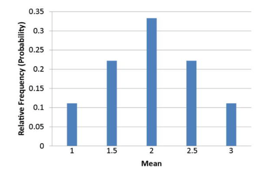
We discussed the probability distribution of the means for the averages of the numbers 1, 2, and 3 picked with replacement, two at a time. That graph is shown below.
Review
To review, see:
3d. Describe a sampling distribution in terms of repeated sampling
- What does it mean to take repeated samples from a population?
- What implication does this have?
Taking the means from repeated samples creates a sampling distribution. Doing this enough times allows you to see the many different results produced by different samples from the same population with the same sample size. You can find the probability of x roughly the same way you found the probability of x in Unit 2.
This is important because statistics is ultimately about making predictions about populations based on a sample (inferential statistics). A major step in calculating margins of error is not only to observe the properties of distributions but also to see how the resulting samples behave.
Review
To review, see:
3e. Compute the mean and standard deviation of the sampling distribution of population proportion p and mean
- What is the sampling distribution of a population proportion, and how does it differ from the sampling distribution of a mean?
- How is the process for finding probabilities different? Can we still use the z-distribution?
Similar to the sampling distribution of the mean, you can take repeated samples from a population where p is the proportion having a certain characteristic, and the sample proportions will be normally distributed if the number sampled each time is sufficiently large.
A good rule of thumb is that given the parameters n (sample size) and p (population proportion), we can use the normal distribution if np and n1-pp are both greater than 10 and p is not too close to 0 or 1. With a very small or large value for p, the distribution becomes right- or left-skewed, and finding areas based on the z-score is unreliable.
The mean ( ) and standard deviation (
}}{\sqrt{n}}") ) formulas use the population proportion
) formulas use the population proportion  rather than the sample proportion
  . This becomes an important difference later when you have to make approximations of the population based on samples and do not have access to the population parameters.
Review
To review, see:
3f. Approximate a sampling distribution based on the properties of the population
How do the properties of the population distribution affect the sampling distribution?
If you have a very large sample size, the short answer is that they do not. The sampling distribution will be bell-shaped and have a predictable mean and standard deviation based on the formulas we discussed earlier in the section on learning outcome 3a.
This explanation does not hold for smaller sample sizes where the properties of the sampling distribution are far less predictable. In some cases, we can come up with sampling distributions and properties through small-sample methods, but these examples are beyond the scope of this course.
Review
To review, see:
3g. Compare the sampling distributions of different sample sizes
- What effect does changing the sample size have on the sampling distribution of a mean?
Keep two things in mind here. First, unless the underlying population distribution is normal, the sample size must be sufficiently large for the sampling distribution to be normal. Second, the standard error (standard deviation of the sample means) becomes smaller with a larger sample. More specifically, it decreases by a factor of the square root of the sample size. For example, if you multiply the sample size by 4, you must divide the standard error by 2 (the square root of 4).
Review
To review, see:
Unit 3 Vocabulary
This vocabulary list includes terms you will need to know to successfully complete the final exam.
- Central Limit Theorem
- sampling distribution
- standard error
Unit 4: Estimation with Confidence Intervals
4a. Compare t-distributions and normal distributions
- What is the difference between a normal distribution and a t-distribution?
- Where would you need to use a t-distribution instead of a normal (x) or the standard normal (z) distribution?
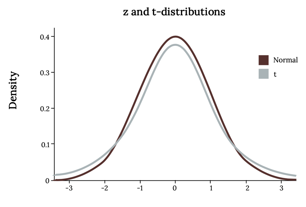
Now, let's introduce the t-distribution, which you can think of as a "brother" to the normal distribution in this hierarchy.
The student's t-distribution is similar to the normal distribution except that it is slightly shorter and flatter, with heavier tails than x or z. In other words, the area to the right of two standard deviations in a normal distribution is 0.025. In a t-distribution, it will be larger. The t-family of distributions is defined by a single parameter called the degrees of freedom, which is symbolized simply as df, although some texts will use other symbols, such as ⋎. When we are talking about the t-distribution, the degrees of freedom are equal to the sample size minus one.
We use the t-distribution in the same situations as the z-distribution. However, we must use t instead when we are unsure of the shape of the population distribution or we are using an estimate of the standard deviation (s instead of σ).
To find an area bound by the t-distribution, we can use technology similar to what we use for the z-distribution. There is a t-distribution table with one row for each of the most common values of t. The drawback is that we cannot use this to find the exact area; only the "t-score" is given for a particular area.
Note that with a t-distribution, as the sample size (thus the degrees of freedom) increases, it is nearly indistinguishable from the z-distribution. In fact, the z-distribution is the t-distribution with an "infinite" degree of freedom! Using the t-distribution gives us a larger margin of error (the range of values above and below a sample statistic that accounts for uncertainty in the estimate) to compensate for the fact that the exact standard deviation of the population is not known.
Review
To review, see:
4b. Describe the performance of different estimators based on their sampling distributions
- What is bias, and how does it differ from accuracy? Can an estimator be biased yet accurate? Can it be inaccurate and unbiased?
- Why is the sample mean considered an unbiased estimator for the population mean?
No estimator is perfect. We use an estimator like a sample mean to give us the best possible estimate of a population mean. However, because of sampling errors, the sample mean will always change for different samples.
Sampling error refers to the fact that, because we do not have access to the entire population, our sample statistics will differ from the population parameters and from each other. If you have a population of size 1,000 with a population mean of 50, you can take five samples of size 20, and because each time you have a different sample, you will get a different sample mean each time, such as {49, 51, 50, 48, 55}.
An unbiased estimator will sometimes estimate too high and sometimes too low, but in the long run, if you average them (the sampling distribution of the mean), you will get a good estimate. In other words, the sample mean is just as likely to overestimate the population mean by 2 as it is to underestimate by 2. A biased estimator might be more likely to overestimate rather than underestimate, or vice versa.
Accuracy differs from bias in that it refers to how much the statistics will differ from the parameter. It's important, but not as much as bias. Accuracy will be better, in general, when we have larger samples, and there is less variance (or standard deviation) in the population.
Review
To review, see:
4c. Calculate confidence intervals for population averages and one population proportion
- What does the confidence interval for a data sample tell you?
- Why was it necessary for you to learn about sampling distributions first?
- How do you calculate a confidence interval?
We use inferential statistics to interpret samples and make conclusions about the population of data. The general method for making these interpretations is roughly the same, whether for population averages, proportions, averages of two different populations, standard deviations, or any other statistic.
Confidence intervals are intervals where we expect to find a population parameter. Think of it as a range of values where we expect the population mean or population proportion to be located. They are calculated at different confidence levels. A 99% confidence interval would have a larger interval, while a 90% confidence interval would be smaller.
First, we find a point estimate, which is usually the sample mean or proportion. Then, given the level of confidence desired, the sample size, and the standard deviation of the population, we can find a margin of error and subtract or add it to the point estimate to get a confidence interval for the population parameter.
When we refer to the level of confidence, we mean the likelihood that our confidence interval contains the true population mean or proportion (or other parameter). Common confidence levels are 90%, 95%, and 99%. A higher confidence level gives a higher likelihood that the interval contains the population parameter. However, the price to be paid is that a higher confidence interval will naturally be wider.
So, for example, we could say there is a 95 percent probability that the population mean is between 10 ± 2.8, or [7.2, 10.8]. If we want to be 99 percent confident, we have to increase the width of the interval, perhaps to 10 ± 3.2. A 100 percent confidence interval is impossible since that would require an infinitely wide margin of error. So there is a give and take. Choosing a confidence level can be more art than science. Balance your desire for accuracy with the need to keep the margin of error low.
You had to learn about sampling distributions first because inferential statistics involves predicting the characteristics of a population based on a sample. To do so, we must first study how those samples behave.
Use the given formulas to calculate the margin of error for the population mean, given a large population (this is when you use the standard normal z-distribution). If the population is small or large and the standard deviation of the population is unknown, you must use Student's t.
The formulas are very similar, except for the distribution. You would use the inverse z-distribution or inverse t-distribution with given degrees of freedom. You also have to plug in the z- or t-score corresponding to ∝/2, where ∝ is equal to the tail area on one side. For example, if you are trying to find a 90 percent confidence interval, that will leave a 10 percent area on the tails, which you divide in half to come up with ∝/2=0.10/2=0.05.
Review
To review, see:
- Basic Sample Statistics and Parameters
- Confidence Interval Simulation
- Confidence Intervals for Correlation and Proportion
4d. Interpret the student-t probability distribution as the sample size changes
- How is the student's t-distribution related to sample size? Why does this not matter for normal or standard normal distributions?
- What happens to the student's t-distribution as the sample size increases? What distribution does it begin to resemble?
The student's t-distribution, like the normal distribution, is a family of distributions defined by one or more parameters. A normal distribution is defined by its mean and standard deviation. The student's t-distribution is defined by the number of degrees of freedom, which is equal to the sample size minus 1.
The larger the sample size, the lower the margin of error, and the larger the degrees of freedom, which combined will give you a smaller margin of error. The larger the degrees of freedom, the more the t-distribution resembles the standard normal (z) distribution. A z-distribution is, by definition, the same as a t-distribution with infinite degrees of freedom!
Review
To review, see:
Unit 4 Vocabulary
This vocabulary list includes terms you will need to know to successfully complete the final exam.
- accuracy
- biased estimator
- confidence interval
- degrees of freedom
- level of confidence
- margin of error
- point estimate
- sampling error
- student's t-distribution
- unbiased estimator
Unit 5: Hypothesis Test
5a. Differentiate between type I and type II errors
- What is an error in the context of hypothesis testing? What is the difference between a Type I and Type II error? How do they relate to each other? Which is more serious?
- How are the Type I and Type II errors calculated or determined?
No hypothesis test is perfect, nor can it produce results that are absolutely 100 percent reliable. This is because the samples are not completely like the population.
- A Type I Error results when the null hypothesis is incorrectly rejected. For our jury example, this means the jury just convicted an innocent defendant.
- A Type II Error is the opposite: failing to detect a difference from the null and incorrectly failing to reject the null hypothesis. For our jury example, the jury failed to convict a guilty defendant.
Remember: the term error does not necessarily mean the researcher made a mistake in their calculation. An error in statistics occurs when we do not have access to the population, and we may, by random chance, get a sample that does not properly represent the population.
For example, a drug study may show that a drug is ineffective simply because a large percentage of the sample the researcher used had a genetic tendency that made the drug less effective. The drug should have shown that it was more effective. A mistake did not cause the error. The sample was unusual. By random chance, the researcher simply chose a group that was less helped by the drug.
Type I and II Errors are related in that, all other things being equal, they are inversely related. The researchers chose the Type I Error (𝛂). They calculate the Type II Error (𝜷) based on possible alternate values for the mean or whatever else they are estimating. When you decrease one, if all else is equal, you inevitably increase the other.
Calculating a Type II Error is beyond the scope of this course. However, this shows why researchers do not simply choose a tiny number for Type I Error: this would increase the Type II Error. Consequently, detecting a true difference from the null will be harder. This creates a more serious situation, although the severity depends on the situation.
For example, in our jury trial scenario, we want to avoid sending an innocent person to prison. Since this is represented by Type I Error, we might consider Type I Error to be more serious and thus lower 𝛂, taking the chance that it will raise 𝜷.
If, in a drug study, the null hypothesis is that a drug is safe for consumption, a Type II error would fail to find that the drug is dangerous, so that would be more serious. In this case, you might choose a more conservative value for alpha, even though it increases the probability that a safe drug will be rejected.
Review
To review, see:
5b. Calculate p-values to be used in hypothesis testing
- What is the p-value in hypothesis testing, and what does it represent?
- What does the p-value tell you about accepting or rejecting the null hypothesis?
The p-value of a hypothesis test provides the key to getting the conclusion of the test. The p-value refers to the probability of obtaining a sample value equal to, or more extreme (see note below) than, the one we got if we assume the null hypothesis is true.
A very low p-value (such as 0.005) means that "if the defendant really is innocent, the probability that we could have obtained the blood and DNA evidence we did is extremely small". This is why a smaller p-value will cause us to reject the null hypothesis.
A very large p-value (usually greater than 0.10) means that, for example, "we assume by default the drug is ineffective; there is a 10 percent chance we could have gotten the results we did even if the drug is ineffective". This is less impressive and might lead us to fail to reject the null hypothesis since we have not found enough evidence to prove the drug is effective.
The proper cutoff (where below would reject the null, and above would fail to reject) is subjective. The standard is 0.05, but can be as low as 0.01 for an aggressive test or as high as 0.10 for a more conservative test.
Note that the definition of extreme depends on whether we are conducting a right-tail test (the probability of a result higher than the result we got), a left-tail test (a lower result), or a two-tail test (higher or lower).
Review
To review, see:
5c. Conduct hypothesis tests for a single population mean and population proportion
- What is hypothesis testing? How is it related to confidence intervals?
- What are a null and an alternative hypothesis?
- How do you know when to use the z- or t-distributions in a hypothesis test for the mean? What about for a proportion?
- Under what circumstances could neither z nor t be used?
Hypothesis testing is a form of inferential statistics similar to confidence intervals. We have a null hypothesis (H0), which we assume to be true by default, and an alternative hypothesis (H1 or Ha), which we can prove or fail to prove based on sample data.
We have three types of alternative hypotheses:
- A right-tailed test has an alternative hypothesis that is greater than the null.
- A left-tailed test has an alternative hypothesis that is less than the null.
- A two-tailed test tests for both higher and lower values than the null. While this may seem more convenient, the downside of a two-tailed test is that it reduces the power of the test, making it less likely to detect a change from the null hypothesis.
The conclusion of a hypothesis test is to reject or fail to reject the null hypothesis. In other words, we assume the null is true, then we either find evidence (based on finding the p-value) that it is false or fail to find evidence that the null is false.
You can think about this situation as a jury trial. The null hypothesis is innocence, and the prosecutor tries to get a guilty verdict by providing evidence that makes the null hypothesis unlikely if all the evidence is true.
You would use either z- or t-distributions based on the same criteria you would use to generate a confidence interval. If you know the population standard deviation and have a reasonably large sample size, you use the z-distribution form of the given equations. If the population standard deviation is unknown or the sample size is small, you would use t.
Remember that the Central Limit Theorem still applies. In other words, if the sample size is small, you must have a normally distributed population, or you cannot use either z or t.
The steps for performing a p-value test are:
- Decide or know what value of Type I Error you will use (𝛂).
- Use the appropriate formula to calculate the test statistic (or test value), which is a calculated value that measures how far the sample data deviates from what would be expected under the null hypothesis. The correct formula is determined by the parameter you are testing (such as mean or proportion) and which distribution you are using (z- or t-test for the mean) within each.
- Use technology or a distribution table to look up the probability of getting a value more than the test value (right-tailed), less than the test value (left-tailed), or a combination of higher and lower (two-tailed). If you are running a two-tailed test, for example, and you get a test value of 1.85, you want to find p(z > 1.85) + p(z < −1.85). This probability is your p-value.
- Compare the p-value to the alpha. If it is lower, reject the null hypothesis; if it is higher, we will fail to reject it.
Remember, we never accept the alternate hypothesis. Just like in a court case, we either find the person guilty (reject the null) or not guilty (fail to reject), but the court never calls the person innocent.
Review
To review, see:
- Setting Up Hypotheses
- Steps and Confidence Intervals in Hypothesis Testing
- Sample Tests for a Population Mean
Unit 5 Vocabulary
This vocabulary list includes terms you will need to know to successfully complete the final exam.
- alternative hypothesis
- left-tailed test
- null hypothesis
- p-value
- right-tailed test
- test statistic
- two-tailed test
- Type I Error
- Type II Error
Unit 6: Linear Regression
6a. Identify the assumptions that inferential statistics in regression are based on
- What are the assumptions about a population we make while conducting inferential statistics?
- Why do we call the regression line the "least squares" regression line?
- What conditions must be true of a sample of points to make the correlation or regression line statistically significant?
There are three assumptions we make while conducting inferential statistics.
- Linearity: We assume the relationship between the variables is linear. We measure the strength of that linear relationship with the correlation coefficient, r.
- Homoscedasticity: This means the variance of the data from the regression line is the same.
- Errors of prediction are normally distributed.
We calculate statistical significance in much the same way as we determine the mean or proportion (from a sample) statistically significant, as we reviewed in Units 4 and 5.
Remember that finding and interpreting the correlation coefficient is always best. While correlation does not necessarily prove a causative relationship between the two variables, if the correlation is very low, it is unlikely that the regression line will be of any use.
As long as the line is non-vertical, you will always get a solution for the least-squares regression line. Think of the phrase, "garbage in, garbage out". If the slope is not significant, then the regression is useless.
The general method behind the regression line formula is to find the line as follows: Draw a vertical line between every point on the scatter plot and the regression line. Then, make that one side of a square. The line that gives the lowest total area (the lowest sum of squares) will be considered the best fit. This process is called least squares regression.
Review
To review, see:
6b. Compute the standard error of a slope
- What does the standard error of a slope tell you?
- How is the standard error computed?
The standard error for a slope tells you basically the same thing that any other standard error tells you. The standard error is the standard deviation of the sampling distribution. So, the standard error for the mean is the standard deviation of a set of sample means. It shows how reliable those samples are by how much the samples vary. A low standard error will produce a narrower confidence interval and make it more likely to reject an incorrect null hypothesis here.
Carry this logic forward to the interpretation of a slope. The standard error may not tell you much by itself (its computation is more complex than for means and proportions), but it is a component of statistical inference involving the slope of a regression line.
The estimated standard error of  is computed using the formula
  , where
  is the standard error of the estimate and
  is the sum of squared deviations of
  from the mean of . is calculated as
 ^{2}") .
.
Review
To review, see:
6c. Test a slope for significance
- How would we test a slope for significance?
- How does this relate to hypothesis testing?
Hypothesis testing works for the slope or correlation of a regression line in the same general way that it works for the mean and proportion: You have a null hypothesis of no significance (r=0) and an alternative that is almost always two-tailed (r≠0). You can use the formulas in the resources below to find the T-statistic and then use the same methods to find the p-value (the combined area of the right and left tails formed by the positive and negative values of that t-statistic).
Review
To review, see:
6d. Construct a confidence interval on a slope
- What should the confidence interval for a slope look like if the slope is significant?
- What is the formula needed to construct a confidence interval for the slope?
Remember, the confidence interval gives the range of values most likely to contain the true parameter. In the case of the slope, we want a confidence interval that does not include 0. If the confidence interval is [-0.8, 2.1], then the slope could be positive or negative, which would cause us to conclude that the slope we found is not significant.
To find a %") confidence interval for the slope
confidence interval for the slope  of the population regression line, use the formula
  and a number of degrees of freedom of
  .
.
Review
To review, see:
6e. Calculate the coefficient of determination and the correlation coefficient
- How is the coefficient of determination calculated?
- How is the correlation coefficient related to the coefficient of determination?
Simply put, the coefficient of determination (a measure of how much of the variation in one variable is explained by another variable in a regression model) is the square of the correlation coefficient. We use the letter  to represent the correlation coefficient and
  to represent the coefficient of determination. So, to calculate the coefficient of determination, square the correlation coefficient.
Review
To review, see:
6f. Interpret the coefficient of determination and the correlation coefficient
- What is the correlation coefficient, and what does it tell us?
- How is the correlation related to the slope of a regression line? Do they tell us roughly the same thing?
- What information does the coefficient of determination tell us?
The correlation coefficient measures the linear relationship between two variables, x and y. It is a number between −1 and 1, inclusive.
- 1 means there is a perfect positive correlation. The scatter plot slopes upward in a straight line.
- −1 means perfect negative correlation. The scatter plot slopes downward in a straight line.
- 0 means there is no correlation, as if every x value produces a completely random value for y.
This way, the correlation coefficient is related to the slope of the regression line because they both have the same sign. The slope will be positive when the correlation is positive, and the slope will be negative when the correlation is negative. However, if the points are in a straight line sloping upward, they will have a correlation coefficient of 1 regardless of the line's slope. Remember, the slope of a line can be any real number, while the correlation coefficient is capped between −1 and +1.
The coefficient of determination tells us, in effect, the proportion of the variable y that is explained by the variable(s) x. So if a correlation is 0.8, then the coefficient of determination is 0.64, telling us that roughly 64% of the dependent variable is explained by the independent variable (x).
Review
To review, see:
Unit 6 Vocabulary
This vocabulary list includes terms you will need to know to successfully complete the final exam.
- coefficient of determination
- correlation coefficient
- homoscedasticity
- least squares regression