Confidence Intervals for the Mean
| Site: | Saylor University |
| Course: | MA121: Introduction to Statistics |
| Book: | Confidence Intervals for the Mean |
| Printed by: | Guest user |
| Date: | Sunday, 21 June 2026, 8:19 AM |
Description
Confidence Intervals Introduction
Say you were interested in the mean weight of 10-year-old girls living in the United States. Since it would have been impractical to weigh all the 10-year-old girls in the United States, you took a sample of 16 and found that the mean weight was 90 pounds. This sample mean of 90 is a point estimate of the population mean. A point estimate by itself is of limited usefulness because it does not reveal the uncertainty associated with the estimate; you do not have a good sense of how far this sample mean may be from the population mean. For example, can you be confident that the population mean is within 5 pounds of 90? You simply do not know.
Confidence intervals provide more information than point estimates. Confidence intervals for means are intervals constructed using a procedure (presented in the next section) that will contain the population mean a specified proportion of the time, typically either 95% or 99% of the time. These intervals are referred to as 95% and 99% confidence intervals respectively. An example of a 95% confidence interval is shown below:

There is good reason to believe that the population mean lies between these two bounds of 72.85 and 107.15 since 95% of the time confidence intervals contain the true mean.
If repeated samples were taken and the 95% confidence interval computed for each sample, 95% of the intervals would contain the population mean. Naturally, 5% of the intervals would not contain the population mean.
It is natural to interpret a 95% confidence interval as an interval with a 0.95 probability of containing the population mean. However, the proper interpretation is not that simple. One problem is that the computation of a confidence interval does not take into account any other information you might have about the value of the population mean. For example, if numerous prior studies had all found sample means above 110, it would not make sense to conclude that there is a 0.95 probability that the population mean is between 72.85 and 107.15. What about situations in which there is no prior information about the value of the population mean? Even here the interpretation is complex. The problem is that there can be more than one procedure that produces intervals that contain the population parameter 95% of the time. Which procedure produces the "true" 95% confidence interval? Although the various methods are equal from a purely mathematical point of view, the standard method of computing confidence intervals has two desirable properties: each interval is symmetric about the point estimate and each interval is contiguous. Recall from the introductory section in the chapter on probability that, for some purposes, probability is best thought of as subjective. It is reasonable, although not required by the laws of probability, that one adopt a subjective probability of 0.95 that a 95% confidence interval, as typically computed, contains the parameter in question.
Confidence intervals can be computed for various parameters, not just the mean. For example, later in this chapter you will see how to compute a confidence interval for  , the population value of Pearson's
  , based on sample data.
Source: David M. Lane , https://onlinestatbook.com/2/estimation/confidence.html![]() This work is in the Public Domain.
This work is in the Public Domain.
Video
Questions
Question 1 out of 2.
Strictly speaking, what is the best interpretation of a 95% confidence interval for the mean?
- If repeated samples were taken and the 95% confidence interval was computed for each sample, 95% of the intervals would contain the population mean.
- A 95% confidence interval has a 0.95 probability of containing the population mean.
- 95% of the population distribution is contained in the confidence interval.
Answers
This is the most accurate interpretation of a 95% confidence interval.
Confidence intervals can be computed for various parameters, not just the mean. Later in this chapter you will see how to compute a confidence interval for the population correlation.
Confidence Interval on the Mean
When you compute a confidence interval on the mean, you compute the mean of a sample in order to estimate the mean of the population. Clearly, if you already knew the population mean, there would be no need for a confidence interval. However, to explain how confidence intervals are constructed, we are going to work backwards and begin by assuming characteristics of the population. Then we will show how sample data can be used to construct a confidence interval.
Assume that the weights of 10-year-old children are normally distributed with a mean of 90 and a standard deviation of 36. What is the sampling distribution of the mean for a sample size of 9? Recall from the section on the sampling distribution of the mean that the mean of the sampling distribution is μ and the standard error of the mean is

For the present example, the sampling distribution of the mean has a mean of 90 and a standard deviation of 36/3 = 12. Note that the standard deviation of a sampling distribution is its standard error. Figure 1 shows this distribution. The shaded area represents the middle 95% of the distribution and stretches from 66.48 to 113.52. These limits were computed by adding and subtracting 1.96 standard deviations to/from the mean of 90 as follows:
90 - (1.96)(12) = 66.48
90 + (1.96)(12) = 113.52
The value of 1.96 is based on the fact that 95% of the area of a normal distribution is within 1.96 standard deviations of the mean; 12 is the standard error of the mean.
Figure 1. The sampling distribution of the mean for N=9. The middle 95% of the distribution is shaded.
Figure 1 shows that 95% of the means are no more than 23.52 units (1.96 standard deviations) from the mean of 90. Now consider the probability that a sample mean computed in a random sample is within 23.52 units of the population mean of 90. Since 95% of the distribution is within 23.52 of 90, the probability that the mean from any given sample will be within 23.52 of 90 is 0.95. This means that if we repeatedly compute the mean (M) from a sample, and create an interval ranging from  to
to  , this interval will contain the population mean 95% of the time. In general, you compute the 95% confidence interval for the mean with the following formula:
Lower limit = 
Upper limit = 
where Z.95 is the number of standard deviations extending from the mean of a normal distribution required to contain 0.95 of the area and σM is the standard error of the mean.
If you look closely at this formula for a confidence interval, you will notice that you need to know the standard deviation ( ) in order to estimate the mean. This may sound unrealistic, and it is. However, computing a confidence interval when σ is known is easier than when σ has to be estimated, and serves a pedagogical purpose. Later in this section we will show how to compute a confidence interval for the mean when σ has to be estimated.
Suppose the following five numbers were sampled from a normal distribution with a standard deviation of 2.5: 2, 3, 5, 6, and 9. To compute the 95% confidence interval, start by computing the mean and standard error:
/5 = 5") .
.
 .
.
 can be found using the normal distribution calculator and specifying that the shaded area is 0.95 and indicating that you want the area to be between the cutoff points. As shown in Figure 2, the value is 1.96. If you had wanted to compute the 99% confidence interval, you would have set the shaded area to 0.99 and the result would have been 2.58.
Figure 2. 95% of the area is between -1.96 and 1.96.
Normal Distribution Calculator
The confidence interval can then be computed as follows:
Lower limit = (1.118)= 2.81")
Upper limit = (1.118)= 7.19")
You should use the t distribution rather than the normal distribution when the variance is not known and has to be estimated from sample data. When the sample size is large, say 100 or above, the t distribution is very similar to the standard normal distribution. However, with smaller sample sizes, the t distribution is leptokurtic, which means it has relatively more scores in its tails than does the normal distribution. As a result, you have to extend farther from the mean to contain a given proportion of the area. Recall that with a normal distribution, 95% of the distribution is within 1.96 standard deviations of the mean. Using the t distribution, if you have a sample size of only 5, 95% of the area is within 2.78 standard deviations of the mean. Therefore, the standard error of the mean would be multiplied by 2.78 rather than 1.96.
The values of t to be used in a confidence interval can be looked up in a table of the t distribution. A small version of such a table is shown in Table 1. The first column,  , stands for degrees of freedom, and for confidence intervals on the mean, is equal to
  , where
  is the sample size.
Table 1. Abbreviated t table.
| df | 0.95 | 0.99 |
|---|---|---|
| 2 | 4.303 | 9.925 |
| 3 | 3.182 | 5.841 |
| 4 | 2.776 | 4.604 |
| 5 | 2.571 | 4.032 |
| 8 | 2.306 | 3.355 |
| 10 | 2.228 | 3.169 |
| 20 | 2.086 | 2.845 |
| 50 | 2.009 | 2.678 |
| 100 | 1.984 | 2.626 |
You can also use the "inverse t distribution" calculator to find the t values to use in confidence intervals. You will learn more about the t distribution in the next section.
Assume that the following five numbers are sampled from a normal distribution: 2, 3, 5, 6, and 9 and that the standard deviation is not known. The first steps are to compute the sample mean and variance:


The next step is to estimate the standard error of the mean. If we knew the population variance, we could use the following formula:
Instead we compute an estimate of the standard error ( ):
):

The next step is to find the value of  . As you can see from Table 1, the value for the 95% interval for
  is 2.776. The confidence interval is then computed just as it is when σM. The only differences are that and rather than
  and
and  are used.
Lower limit = (1.225) = 1.60")
Upper limit = (1.225) = 8.40")
More generally, the formula for the 95% confidence interval on the mean is:
Lower limit = (s_M)")
Upper limit = (sM)")
where  is the sample mean,
  is the t for the confidence level desired (0.95 in the above example), and is the estimated standard error of the mean.
We will finish with an analysis of the Stroop Data. Specifically, we will compute a confidence interval on the mean difference score. Recall that 47 subjects named the color of ink that words were written in. The names conflicted so that, for example, they would name the ink color of the word "blue" written in red ink. The correct response is to say "red" and ignore the fact that the word is "blue." In a second condition, subjects named the ink color of colored rectangles.
| Naming Colored Rectangle | Interference | Difference |
|---|---|---|
| 17 | 38 | 21 |
| 15 | 58 | 43 |
| 18 | 35 | 17 |
| 20 | 39 | 19 |
| 18 | 33 | 15 |
| 20 | 32 | 12 |
| 20 | 45 | 25 |
| 19 | 52 | 33 |
| 17 | 31 | 14 |
| 21 | 29 | 8 |
Table 2 shows the time difference between the interference and color-naming conditions for 10 of the 47 subjects. The mean time difference for all 47 subjects is 16.362 seconds and the standard deviation is 7.470 seconds. The standard error of the mean is 1.090. A table shows the critical value of for 47 - 1 = 46 degrees of freedom is 2.013 (for a 95% confidence interval). Therefore the confidence interval is computed as follows:
Lower limit = 16.362 - (2.013)(1.090) = 14.17
Upper limit = 16.362 + (2.013)(1.090) = 18.56
Therefore, the interference effect (difference) for the whole population is likely to be between 14.168 and 18.555 seconds.
R code
Make sure to put the data file in the default directory.
data=read.csv(file="stroop.csv")
data$diff = data$interfer-data$colors
t.test(data$diff)
[1] 14.16842 18.55498
attr(,"conf.level")
[1] 0.95
Video
Questions
Question 1 out of 5.
You know the mean and standard deviation of the population. You take a sample from this population and compute the 90% confidence interval for the mean. This interval contains values that are within how many standard deviations of the mean?
Question 2 out of 5.
There is a population of test scores. You take a sample of 11 scores and use them to estimate the population mean and standard deviation. Then you compute a 95% confidence interval for the mean. This confidence interval contains values that are within how many standard deviations of its mean?
Question 3 out of 5.
You take a sample (N = 25) of test scores from a population. The sample mean is 38, and the population standard deviation is 6.5. What is the 95% confidence interval on the mean?
- (37.49, 38.51)
- (36.49, 39.51)
- (35.45, 40.55)
- (25.26, 50.74)
Question 4 out of 5.
You take a sample (N = 9) of heights of fifth graders. The sample mean was 49, and the sample standard deviation was 4. What is the 99% confidence interval on the mean?
- (39.76, 58.24)
- (44.53, 53.47)
- (45.93, 52.07)
- (47.51, 50.49)
Question 5 out of 5.
Based on the data below, what is the upper limit of
the 95% confidence interval for the mean of A1? You may want to use the
Analysis Lab or another statistical program to answer this.
________
A1
  1
  4
  5
  5
  7
  9
 10
 11
 12
 13
 14
 14
 17
 19
 20
 23
 24
 24
 24
 29
Answers
Because you know the standard deviation of the population, you can use the normal distribution. If you use the normal distribution calculator, you will find that 90% of the area is within 1.65 standard deviations of the mean.
You have to estimate the standard deviation of the population, so you need to use the t distribution. Because your sample size is 11, your degrees of freedom are 11 - 1 = 10. Looking at the t distribution table, you can see that 95% of the distribution falls within 2.23 standard deviations of the mean.
First, the standard error of the mean is 6.5/5 = 1.3. Second, you know the population standard deviation, so you can use the normal distribution. 95% of the distribution lies within 1.96 standard deviations of the mean. Lower limit: 38 - (1.3)(1.96) = 35.45; Upper limit: 38 + (1.3)(1.96) = 40.55
In this case, the population standard deviation is unknown, so you need to use the t distribution (df = N-1 = 9-1 = 8). From the t distribution table, you see that 99% of the distribution lies within 3.355 standard deviations of the mean when t has 8 degrees of freedom. The standard error of the mean = 4/3 = 1.333. Lower limit: 49 - (1.333)(3.355) = 44.53; Upper limit: 49 + (1.333)(3.355) = 53.47
Use a statistical program to compute the 95% CI. To compute it by hand, you need the sample mean and standard error and the t value for 19 df. 14.25 + (2.093)(1.784) = 17.984
t Distribution
In the introduction to normal distributions it was shown that 95% of the area of a normal distribution is within 1.96 standard deviations of the mean. Therefore, if you randomly sampled a value from a normal distribution with a mean of 100, the probability it would be within  of 100 is 0.95. Similarly, if you sample values from the population, the probability that the sample mean () will be within
  of 100 is 0.95.
Now consider the case in which you have a normal distribution but you do not know the standard deviation. You sample values and compute the sample mean () and estimate the standard error of the mean (") with . What is the probability that will be within
with . What is the probability that will be within  of the population mean (
 )? This is a difficult problem because there are two ways in which could be more than
  from : (1) could, by chance, be either very high or very low and (2) could, by chance, be very low. Intuitively, it makes sense that the probability of being within 1.96 standard errors of the mean should be smaller than in the case when the standard deviation is known (and cannot be underestimated). But exactly how much smaller? Fortunately, the way to work out this type of problem was solved in the early 20th century by W. S. Gosset who determined the distribution of a mean divided by an estimate of its standard error. This distribution is called the Student's distribution or sometimes just the distribution. Gosset worked out the distribution and associated statistical tests while working for a brewery in Ireland. Because of a contractual agreement with the brewery, he published the article under the pseudonym "Student". That is why the test is called the "Student's test".
The distribution is very similar to the normal distribution when the estimate of variance is based on many degrees of freedom, but has relatively more scores in its tails when there are fewer degrees of freedom. Figure 1 shows t distributions with 2, 4, and 10 degrees of freedom and the standard normal distribution. Notice that the normal distribution has relatively more scores in the center of the distribution and the t distribution has relatively more in the tails. The t distribution is therefore leptokurtic. The distribution approaches the normal distribution as the degrees of freedom increase.
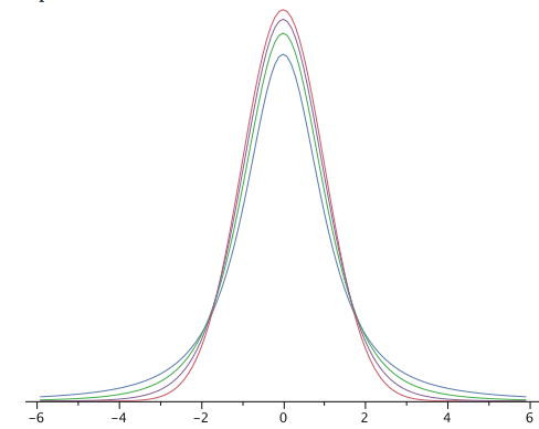
Figure 1. A comparison of distributions with 2, 4, and 10 and the standard normal distribution. The distribution with the lowest peak is the 2 distribution, the next lowest is 4 , the lowest after that is 10 , and the highest is the standard normal distribution.
Since the t distribution is leptokurtic, the percentage of the distribution within 1.96 standard deviations of the mean is less than the 95% for the normal distribution. Table 1 shows the number of standard deviations from the mean required to contain 95% and 99% of the area of the t distribution for various degrees of freedom. These are the values of that you use in a confidence interval. The corresponding values for the normal distribution are 1.96 and 2.58 respectively. Notice that with few degrees of freedom, the values of t are much higher than the corresponding values for a normal distribution and that the difference decreases as the degrees of freedom increase. The values in Table 1 can be obtained from the "Find t for a confidence interval" calculator.
Table 1. Abbreviated t table.
| df | 0.95 | 0.99 |
|---|---|---|
| 2 | 4.303 | 9.925 |
| 3 | 3.182 | 5.841 |
| 4 | 2.776 | 4.604 |
| 5 | 2.571 | 4.032 |
| 8 | 2.306 | 3.355 |
| 10 | 2.228 | 3.169 |
| 20 | 2.086 | 2.845 |
| 50 | 2.009 | 2.678 |
| 100 | 1.984 | 2.626 |
Returning to the problem posed at the beginning of this section, suppose you sampled 9 values from a normal population and estimated the standard error of the mean () with . What is the probability that would be within  of ? Since the sample size is 9, there are
  . From Table 1 you can see that with 8 the probability is 0.95 that the mean will be within 2.306 of . The probability that it will be within 1.96 of is therefore lower than 0.95.
As shown in Figure 2, the "t distribution" calculator can be used to find that 0.086 of the area of a distribution is more than 1.96 standard deviations from the mean, so the probability that would be less than from is 1 - 0.086 = 0.914.
Figure 2. Area more than 1.96 standard deviations from the mean in a distribution with 8 . Note that the two-tailed button is selected so that the area in both tails will be included.
As expected, this probability is less than 0.95 that would have been obtained if had been known instead of estimated.
Video
Questions
Question 1 out of 5.
Select all of the following that are correct descriptions of the t distribution.
- There are more scores in the tails than in a normal distribution.
- There are more scores in the center than in a normal distribution.
- It is leptokurtic.
- You use it when you do not know the population standard deviation.
- A t distribution with 20 degrees of freedom has 95% of its distribution within 1.96 standard deviations of its mean.
Question 2 out of 5.
A t distribution with which of the following degrees of freedom is the closest to a normal distribution?
- 0
- 2
- 12
- 50
Question 3 out of 5.
For a t distribution with 15 degrees of freedom, 90% of the distribution is within how many standard deviations of the mean?
Question 4 out of 5.
In a t distribution with 10 degrees of freedom, what is the probability of getting a value within two standard deviations of the mean?
Question 5 out of 5.
There is a population of test scores with an unknown standard deviation. You sample 21 scores from this population, and you calculate the mean and standard deviation. You get a value for the mean that is 1.5 standard errors greater than what you think is the population mean. What is the probability that you would get a value 1.5 standard deviations or more from the mean in this t distribution?
Answers
A t distribution has more scores in its tails and fewer in the center than a normal distribution, so it is leptokurtic. Also, a t distribution with 20 degrees of freedom has 95% of its distribution within 2.086 standard deviations of its mean.
As the degrees of freedom increase, the t distribution looks more and more like a normal distribution.
Use the "Find t for a confidence interval" calculator for a 90% confidence interval and you will get 1.753.
Use the "t distribution" calculator and enter 10 for df and 2 for t. You will see that the probability of getting something greater than 2 SDs from the mean is .0734, so the probability of getting something less than 2 SDs from the mean is 1 - .0734 = .9266.
There is a population of test scores with an unknown standard deviation. You sample 21 scores from this population, and you calculate the mean and standard deviation. You get a value for the mean that is 1.5 standard errors greater than what you think is the population mean. What is the probability that you would get a value 1.5 standard deviations or more from the mean in this t distribution? Answer: 0.148 or 14.8%
Difference between Means
It is much more common for a researcher to be interested in the difference between means than in the specific values of the means themselves. We take as an example the data from the "Animal Research" case study. In this experiment, students rated (on a 7-point scale) whether they thought animal research is wrong. The sample sizes, means, and variances are shown separately for males and females in Table 1.
Table 1. Means and Variances in Animal Research study.
| Condition | n | Mean | Variance |
|---|---|---|---|
| Females | 17 | 5.353 | 2.743 |
| Males | 17 | 3.882 | 2.985 |
As you can see, the females rated animal research as more wrong than did the males. This sample difference between the female mean of 5.35 and the male mean of 3.88 is 1.47. However, the gender difference in this particular sample is not very important. What is important is the difference in the population. The difference in sample means is used to estimate the difference in population means. The accuracy of the estimate is revealed by a confidence interval.
In order to construct a confidence interval, we are going to make three assumptions:
- The two populations have the same variance. This assumption is called the assumption of homogeneity of variance.
- The populations are normally distributed.
- Each value is sampled independently from each other value.
The consequences of violating these assumptions are discussed in a later section. For now, suffice it to say that small-to-moderate violations of assumptions 1 and 2 do not make much difference.
A confidence interval on the difference between means is computed using the following formula:
Lower Limit = (S_{M_1-M_2})")
Upper Limit = (S_{M_1-M_2})")
where  is the difference between sample means,
is the t for the desired level of confidence, and
is the difference between sample means,
is the t for the desired level of confidence, and  is the estimated standard
error of the difference between sample means. The meanings
of these terms will be made clearer as the calculations are demonstrated.
is the estimated standard
error of the difference between sample means. The meanings
of these terms will be made clearer as the calculations are demonstrated.
We continue to use the data from the "Animal Research" case study and will compute a confidence interval on the difference between the mean score of the females and the mean score of the males. For this calculation, we will assume that the variances in each of the two populations are equal.
The first step is to compute the estimate of the
standard error of the difference between means ") .
Recall from the relevant
section in the chapter on sampling distributions that the
formula for the standard error of the difference in means in the
population is:
.
Recall from the relevant
section in the chapter on sampling distributions that the
formula for the standard error of the difference in means in the
population is:

In order to estimate this quantity, we estimate
 and use that estimate in place
of . Since we are assuming the
population variances are the same, we estimate this variance by
averaging our two sample variances. Thus, our estimate of variance
is computed using the following formula:
and use that estimate in place
of . Since we are assuming the
population variances are the same, we estimate this variance by
averaging our two sample variances. Thus, our estimate of variance
is computed using the following formula:

here MSE is our estimate of σ2. In this example,
/2 = 2.864") .
.
Note that MSE stands for "mean square error" and is the mean squared deviation of each score from its group's mean.
Since  (the number of scores in
each condition) is 17,
(the number of scores in
each condition) is 17,
(2.864)}{17}} = 0.5805") .
.
The next step is to find the t to use for the
confidence interval (). To calculate
, we need to know the degrees
of freedom. The degrees of freedom is the number of
independent estimates of variance on which MSE is based. This
is equal to  + (n_2
- 1)") where
where  is the sample size of the
first group and
is the sample size of the
first group and  is the sample size
of the second group. For this example,
is the sample size
of the second group. For this example,  . When
  , it is conventional to use ""
to refer to the sample size of each group. Therefore, the degrees
of freedom is 16 + 16 = 32.
, it is conventional to use ""
to refer to the sample size of each group. Therefore, the degrees
of freedom is 16 + 16 = 32.
From either the above calculator or a table, you can find that
the for a 95% confidence interval for  is 2.037.
We now have all the components needed to compute the confidence interval. First, we know the difference between means:

We know the standard error of the difference between means is

and that the for the 95% confidence interval
with is

Therefore, the 95% confidence interval is
Lower Limit = (0.5805) = 0.29")
Upper Limit = (0.5805) = 2.65")
We can write the confidence interval as:

where  is the population mean for
females and
is the population mean for
females and  is the population mean
for males. This analysis provides evidence that the mean for females
is higher than the mean for males, and that the difference between
means in the population is likely to be between 0.29 and 2.65.
is the population mean
for males. This analysis provides evidence that the mean for females
is higher than the mean for males, and that the difference between
means in the population is likely to be between 0.29 and 2.65.
Formatting data for Computer Analysis
Most computer programs that compute tests require
your data to be in a specific form. Consider the data in Table 2.
Table 2. Example Data.
| Group 1 | Group 2 |
|---|---|
| 3 | 5 |
| 4 | 6 |
| 5 | 7 |
Here there are two groups, each with three observations. To format
these data for a computer program, you normally have to use two
variables: the first specifies the group the subject is in and the
second is the score itself. For the data in Table 2, the reformatted
data look as follows:
Table 3. Reformatted Data.
| G | Y |
|---|---|
| 1 | 3 |
| 1 | 4 |
| 1 | 5 |
| 2 | 5 |
| 2 | 6 |
| 2 | 7 |
To use Analysis Lab to do the calculations, you would copy the data and then
- Click the "Enter/Edit User Data" button. (You may be warned that for security reasons you must use the keyboard shortcut for pasting data).
- Paste your data.
- Click "Accept Data".
- Set the Dependent Variable to Y.
- Set the Grouping Variable to G.
- Click the t-test confidence interval button.
The 95% confidence interval on the difference between means extends from -4.267 to 0.267.
Computations for Unequal Sample Sizes (optional)
The calculations are somewhat more
complicated when the sample sizes are not equal. One consideration
is that MSE, the estimate of variance, counts the sample with
the larger sample size more than the sample with the smaller sample
size. Computationally this is done by computing the sum of squares
error (SSE) as follows:
^2 + \Sigma (X - M_2)^2")
where  is the mean for group 1 and
 is the mean for group 2. Consider
the following small example:
is the mean for group 2. Consider
the following small example:
Table 4. Example Data.
| Group 1 | Group 2 |
|---|---|
| 3 | 2 |
| 4 | 4 |
| 5 |
 and
and  .
.
^2 + (4-4)^2 + (5-4)^2 + (2-3)^2 + (4-3)^2 = 4")
Then, MSE is computed by: 
where the degrees of freedom () is computed as before:
 + (n_2 -1) = (3-1) + (2-1) = 3") .
.
 .
.
The formula

is replaced by

where  is the harmonic mean of the sample sizes and is computed
as follows:
is the harmonic mean of the sample sizes and is computed
as follows:

and
(1.333)}{2.4}} = 1.054") .
.
for 3 and the 0.05 level = 3.182.
Therefore the 95% confidence interval is
Lower Limit = (1.054)= -2.35")
Upper Limit = (1.054)= 4.35")
We can write the confidence interval as:

Video
Questions
Question 1 out of 4.
Select all of the assumptions that you need to make when creating a confidence interval on the difference between means.
- At least 2% of the population sampled
- Independently sampled values
- Homogeneity of variance
- Normally distributed populations
Question 2 out of 4.
You are comparing men and women on hours spent watching TV. You pick a sample of 12 men and 14 women and calculate a confidence interval on the difference between means. How many degrees of freedom does your t value have?
Question 3 out of 4.
You are comparing freshmen and seniors at your college on hours spent studying per day. You pick a sample of 11 people from each group. For freshmen, the mean was 3 and the variance was 1.2. For seniors, the mean was 2 and the variance was 1. Calculate a 90% confidence interval on the difference between means (freshmen - seniors). What is the lower limit of this CI?
Question 4 out of 4.
Scores on a test taken by 1st graders and 2nd graders were compared to look at development. The five 1st graders sampled got the following scores: 4, 3, 5, 7, 4. The five 2nd graders sampled got the following scores: 7, 9, 8, 6, 9. Compute the 95% confidence interval for the difference between means (2nd graders - 1st graders). You may use the Analysis Lab. What is the upper limit?
Grade	Score
  1	  4
  1	  3
  1	  5
  1	  7
  1	  4
  2	  7
  2	  9
  2	  8
  2	  6
  2	  9
Answers
You assume that the values were sampled independently of each other, the populations have the same variance (homogeneity of variance), and the populations are normally distributed.
df = (n1 - 1) + (n2 - 1) = (12 - 1) + (14 -1) = 24
Difference between means = 3 - 2 = 1; MSE = (1 + 1.2)/2 = 1.1; Standard error = sqrt(2(1.1)/11) = .447; df = 20; t = 1.725; Lower limit = 1 - (1.725)(.447) = 0.229
Enter this data into the Analysis Lab (or another statistical program). Your grouping variable (grade) should be composed of all 1's (1st graders) and 2's (2nd graders), and your dependent variable should contain the test scores. You should get the following confidence interval: (1.137, 5.263). If the statistical program calculates the mean of 1st - 2nd graders, you will have to reverse the confidence interval it gives you.