Statistical Inference about Slope

Site:	Saylor Academy
Course:	MA121: Introduction to Statistics
Book:	Statistical Inference about Slope

Printed by:	Guest user
Date:	Wednesday, 6 May 2026, 2:15 PM

Description

This is a book resource with multiple pages. Navigate between the pages using the buttons.

Statistical Inferences About β1

Statistical Inferences About β1

This section details two types of inferences on the slope parameter, considering both confidence intervals and hypothesis testing. Complete the odd-numbered exercises at the end of the section before checking your answers.

The parameter $β_1$ , the slope of the population regression line, is of primary importance in regression analysis because it gives the true rate of change in the mean $E(y)$ in response to a unit increase in the predictor variable $x$ . For every unit increase in $x$ the mean of the response variable y changes by $β_1$ units, increasing if $β_1 > 0$ and decreasing if $β_1 < 0$ . We wish to construct confidence intervals for $β_1$ and test hypotheses about it.

Confidence Intervals for $β_1$

The slope $\hat{\beta}_{1}$ of the least squares regression line is a point estimate of $β_1$ . A confidence interval for $β_1$ is given by the following formula.

100(1−α)% Confidence Interval for the Slope $β_1$ of the Population Regression Line

$\hat{\beta}_{1} \pm t_{\alpha / 2} \frac{s_{\varepsilon}}{\sqrt{S S_{x x}}}$

where $\hat{\beta}_{1} \pm t_{\alpha / 2} \frac{s_{\varepsilon}}{\sqrt{S S_{x x}}}$ and the number of degrees of freedom is $df=n−2$ .

The assumptions listed in Section 10.3 "Modelling Linear Relationships with Randomness Present" must hold.

Definition

The statistic sε is called the sample standard deviation of errors. It estimates the standard deviation σ of the errors in the population of y-values for each fixed value of $x$ (see Figure 10.5 "The Simple Linear Model Concept" in Section 10.3 "Modelling Linear Relationships with Randomness Present").

Example 6

Construct the 95% confidence interval for the slope $β_1$ of the population regression line based on the five-point sample data set

$\begin{array}{c|ccccc}x & 2 & 2 & 6 & 8 & 10 \\\hline y & 0 & 1 & 2 & 3 & 3\end{array}$

Solution:

The point estimate $\hat{\beta}_{1}$ of $β_1$ was computed in Note 10.18 "Example 2" in Section 10.4 "The Least Squares Regression Line" as $\hat{\beta}_{1}=0.34375$ . In the same example $SS_{xx}$ was found to be $SS_{xx}=51.2$ . The sum of the squared errors $SSE$ was computed in Note 10.23 "Example 4" in Section 10.4 "The Least Squares Regression Line" as $SSE=0.75$ . Thus

style="text-align: center;"> $s_{\varepsilon}=\sqrt{\frac{S S E}{n-2}}=\sqrt{\frac{0.75}{3}}=0.50$

Confidence level 95% means $α=1−0.95=0.05$ so $α∕2=0.025$ . From the row labeled $df=3$ in Figure 12.3 "Critical Values of " we obtain $t_{0.025}=3.182$ . Therefore

$\hat{\beta}_{1} \pm t_{\alpha / 2} \frac{s_{\varepsilon}}{\sqrt{S S_{x x}}}=0.34375 \pm 3.182\left(\frac{0.50}{\sqrt{51.2}}\right)=0.34375 \pm 0.2223$

which gives the interval (0.1215,0.5661). We are 95% confident that the slope $β_1$ of the population regression line is between 0.1215 and 0.5661.

Example 7

Using the sample data in Table 10.3 "Data on Age and Value of Used Automobiles of a Specific Make and Model" construct a 90% confidence interval for the slope $β_1$ of the population regression line relating age and value of the automobiles of Note 10.19 "Example 3" in Section 10.4 "The Least Squares Regression Line". Interpret the result in the context of the problem.

Solution:

The point estimate $\hat{\beta}_{1}$ if $β_1$ was computed in Note 10.19 "Example 3", as was $SS_{xx}$ . Their values are $\hat{\beta}_{1}=−2.05$ and $SS_{xx}=14$ . The sum of the squared errors $SSE$ was computed in Note 10.24 "Example 5" in Section 10.4 "The Least Squares Regression Line" as $SSE=28.946$ . Thus

$s_{\varepsilon}=\sqrt{\frac{S S E}{n-2}}=\sqrt{\frac{28.946}{8}}=1.902169814$

Confidence level 90% means $α=1−0.90=0.10$ so $α∕2=0.05$ . From the row labeled $df=8$ in Figure 12.3 "Critical Values of " we obtain $t_{0.05}=1.860$ . Therefore

$\hat{\beta}_{1} \pm t_{\alpha / 2} \frac{s_{\varepsilon}}{\sqrt{S S_{x x}}}=-2.05 \pm 1.860\left(\frac{1.902169814}{\sqrt{14}}\right)=-2.05 \pm 0.95$

which gives the interval (−3.00,−1.10). We are 90% confident that the slope $β_1$ of the population regression line is between −3.00 and −1.10. In the context of the problem this means that for vehicles of this make and model between two and six years old we are 90% confident that for each additional year of age the average value of such a vehicle decreases by between $1,100 and $3,000.

Testing Hypotheses About $β_1$

Hypotheses regarding $β_1$ can be tested using the same five-step procedures, either the critical value approach or the p-value approach, that were introduced in Section 8.1 "The Elements of Hypothesis Testing" and Section 8.3 "The Observed Significance of a Test" of Chapter 8 "Testing Hypotheses". The null hypothesis always has the form $H_0: β_1 = B_0$ where $B_0$ is a number determined from the statement of the problem. The three forms of the alternative hypothesis, with the terminology for each case, are:

Form of $H_a$	Terminology
$H_a: β_1 < B_0$	Left-tailed
$H_a: β_1 > B_0$	Right-tailed
$H_a: β_1 ≠ B_0$	Two-tailed

The value zero for $B_0$ is of particular importance since in that case the null hypothesis is $H_0: β_1 = 0$ , which corresponds to the situation in which x is not useful for predicting y. For if $β_1=0$ then the population regression line is horizontal, so the mean $E(y)$ is the same for every value of $x$ and we are just as well off in ignoring $x$ completely and approximating $y$ by its average value. Given two variables $x$ and $y$ , the burden of proof is that $x$ is useful for predicting $y$ , not that it is not. Thus the phrase "test whether $x$ is useful for prediction of $y$ ," or words to that effect, means to perform the test

$H_0: β_1 = 0$ vs. $H_a: β_1 ≠ 0$

Standardized Test Statistic for Hypothesis Tests Concerning the Slope $β_1$ of the Population Regression Line

$T=\frac{\hat{\beta}_{1}-B_{0}}{s_{\varepsilon} / \sqrt{S S_{x x}}}$

The test statistic has Student's t-distribution with $df=n−2$ degrees of freedom.

The assumptions listed in Section 10.3 "Modelling Linear Relationships with Randomness Present" must hold.

Example 8

Test, at the 2% level of significance, whether the variable x is useful for predicting y based on the information in the five-point data set

$\begin{array}{c|ccccc}x & 2 & 2 & 6 & 8 & 10 \\\hline y & 0 & 1 & 2 & 3 & 3\end{array}$

Solution:

We will perform the test using the critical value approach.

Step 1. Since $x$ is useful for prediction of $y$ precisely when the slope $β_1$ of the population regression line is nonzero, the relevant test is

$H_0: β_1=0$
vs. $H_a: β_1 ≠ 0$ @ $α=0.02$

Step 2. The test statistic is

$T=\frac{\hat{\beta}_{1}}{s_{\varepsilon} / \sqrt{S S_{x x}}}$

and has Student's t-distribution with $n−2=5−2=3$ degrees of freedom.

Step 3. From Note 10.18 "Example 2", $\hat{\beta}_{1}=0.34375$ and $SS_{xx}=51.2$ . From Note 10.30 "Example 6", $sε=0.50$ . The value of the test statistic is therefore

$T=\frac{\hat{\beta}_{1}-B_{0}}{s_{\varepsilon} / \sqrt{S S_{x x}}}=\frac{0.34375}{0.50 / \sqrt{51.2}}=4.919$

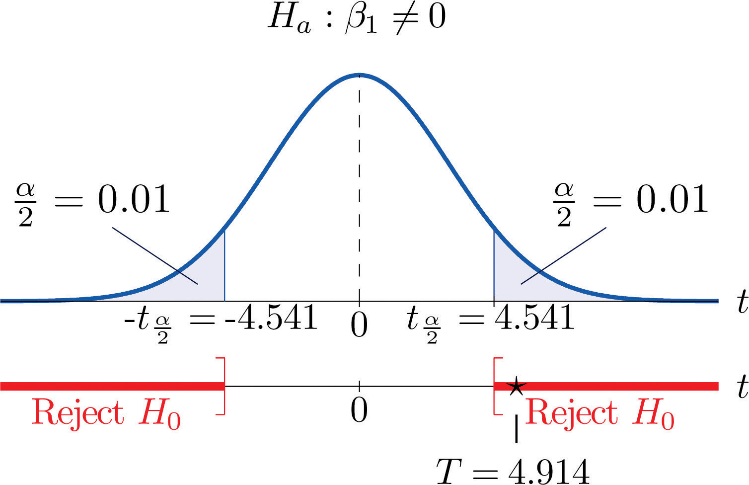
Step 4. Since the symbol in $H_a$ is "≠" this is a two-tailed test, so there are two critical values $±t_{α∕2} = ± t_{0.01}$ . Reading from the line in Figure 12.3 "Critical Values of " labeled $df=3$ , $t_{0.01}=4.541$ . The rejection region is $(−∞,−4.541] ∪ [4.541,∞)$ .

Step 5. As shown in Figure 10.9 "Rejection Region and Test Statistic for " the test statistic falls in the rejection region. The decision is to reject $H_0$ . In the context of the problem our conclusion is:

The data provide sufficient evidence, at the 2% level of significance, to conclude that the slope of the population regression line is nonzero, so that $x$ is useful as a predictor of $y$ .

Figure 10.9 Rejection Region and Test Statistic for Note 10.33 "Example 8"

Example 9

A car salesman claims that automobiles between two and six years old of the make and model discussed in Note 10.19 "Example 3" in Section 10.4 "The Least Squares Regression Line" lose more than $1,100 in value each year. Test this claim at the 5% level of significance.

Solution:

We will perform the test using the critical value approach.

Step 1. In terms of the variables $x$ and $y$ , the salesman's claim is that if $x$ is increased by 1 unit (one additional year in age), then y decreases by more than 1.1 units (more than $1,100). Thus his assertion is that the slope of the population regression line is negative, and that it is more negative than −1.1. In symbols, $β_1 < −1.1$ . Since it contains an inequality, this has to be the alternative hypotheses. The null hypothesis has to be an equality and have the same number on the right hand side, so the relevant test is

$H_0: β_1=−1.1$

vs. $H_α: β_1 < −1.1$ @ $α=0.05$

Step 2. The test statistic is

$T=\frac{\hat{\beta}_{1}-B_{0}}{s_{\varepsilon} / \sqrt{S S_{x x}}}$

and has Student's t-distribution with 8 degrees of freedom.

Step 3. From Note 10.19 "Example 3", $\hat{\beta}_{1}=−2.05$ and $SS_{xx}=14$ . From Note 10.31 "Example 7", $sε=1.902169814$ . The value of the test statistic is therefore

$T=\frac{\hat{\beta}_{1}-B_{0}}{s_{\varepsilon} / \sqrt{S S_{x x}}}=\frac{-2.05-(-1.1)}{1.902169814 / \sqrt{14}}=-1.869$

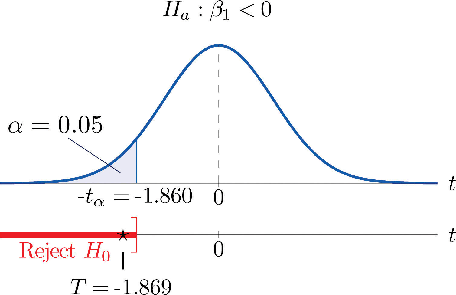
Step 4. Since the symbol in $H_a$ is "<" this is a left-tailed test, so there is a single critical value $−t_α=−t_{0.05}$ . Reading from the line in Figure 12.3 "Critical Values of " labeled $df=8$ , $t_{0.05}=1.860$ . The rejection region is (−∞,−1.860].

Step 5. As shown in Figure 10.10 "Rejection Region and Test Statistic for " the test statistic falls in the rejection region. The decision is to reject $H_0$ . In the context of the problem our conclusion is:

The data provide sufficient evidence, at the 5% level of significance, to conclude that vehicles of this make and model and in this age range lose more than $1,100 per year in value, on average.

Figure 10.10 Rejection Region and Test Statistic for Note 10.34 "Example 9"

This text was adapted by Saylor Academy under a Creative Commons Attribution-NonCommercial-ShareAlike 3.0 License without attribution as requested by the work's original creator or licensor.

Key Takeaways

The parameter $β_1$ , the slope of the population regression line, is of primary interest because it describes the average change in $y$ with respect to unit increase in $x$ .
The statistic $\hat{\beta}_{1}$ , the slope of the least squares regression line, is a point estimate of $β_1$ . Confidence intervals for $β_1$ can be computed using a formula.
Hypotheses regarding $β_1$ are tested using the same five-step procedures introduced in Chapter 8 "Testing Hypotheses".

Exercises

For the Basic and Application exercises in this section use the computations that were done for the exercises with the same number in Section 10.2 "The Linear Correlation Coefficient" and Section 10.4 "The Least Squares Regression Line".

1. Construct the 95% confidence interval for the slope $β_1$ of the population regression line based on the sample data set of Exercise 1 of Section 10.2 "The Linear Correlation Coefficient".

3. Construct the 90% confidence interval for the slope $β_1$ of the population regression line based on the sample data set of Exercise 3 of Section 10.2 "The Linear Correlation Coefficient".

5. For the data in Exercise 5 of Section 10.2 "The Linear Correlation Coefficient" test, at the 10% level of significance, whether $x$ is useful for predicting $y$ (that is, whether $β_1≠0$ ).

7. Construct the 90% confidence interval for the slope $β_1$ of the population regression line based on the sample data set of Exercise 7 of Section 10.2 "The Linear Correlation Coefficient".

9. For the data in Exercise 9 of Section 10.2 "The Linear Correlation Coefficient" test, at the 1% level of significance, whether x is useful for predicting $y$ (that is, whether $β_1≠0$ ).

Applications

11. For the data in Exercise 11 of Section 10.2 "The Linear Correlation Coefficient" construct a 90% confidence interval for the mean number of new words acquired per month by children between 13 and 18 months of age.

13. For the data in Exercise 13 of Section 10.2 "The Linear Correlation Coefficient" test, at the 10% level of significance, whether age is useful for predicting resting heart rate.

15. For the situation described in Exercise 15 of Section 10.2 "The Linear Correlation Coefficient"

Construct the 95% confidence interval for the mean increase in revenue per additional thousand dollars spent on advertising.
An advertising agency tells the business owner that for every additional thousand dollars spent on advertising, revenue will increase by over $25,000. Test this claim (which is the alternative hypothesis) at the 5% level of significance.
Perform the test of part (b) at the 10% level of significance.
Based on the results in (b) and (c), how believable is the ad agency’s claim? (This is a subjective judgement.)

17. For the data in Exercise 17 of Section 10.2 "The Linear Correlation Coefficient" test, at the 10% level of significance, whether course average before the final exam is useful for predicting the final exam grade.

19. For the data in Exercise 19 of Section 10.2 "The Linear Correlation Coefficient" test, at the 1/10th of 1% level of significance, whether, ignoring all other facts such as age and body mass, the amount of the medication consumed is a useful predictor of blood concentration of the active ingredient.

21. For the data in Exercise 21 of Section 10.2 "The Linear Correlation Coefficient"

Construct the 95% confidence interval for the mean increase in strength at 28 days for each additional hundred psi increase in strength at 3 days.
Test, at the 1/10th of 1% level of significance, whether the 3-day strength is useful for predicting 28-day strength.

Large Data Set Exercises

23. Large Data Set 1 lists the SAT scores and GPAs of 1,000 students.

http://www.gone.2012books.lardbucket.org/sites/all/files/data1.xls

Compute the 90% confidence interval for the slope $β_1$ of the population regression line with SAT score as the independent variable $(x)$ and GPA as the dependent variable $(y)$ .
Test, at the 10% level of significance, the hypothesis that the slope of the population regression line is greater than 0.001, against the null hypothesis that it is exactly 0.001.

25. Large Data Set 13 records the number of bidders and sales price of a particular type of antique grandfather clock at 60 auctions.

http://www.gone.2012books.lardbucket.org/sites/all/files/data13.xls

Compute the 95% confidence interval for the slope $β_1$ of the population regression line with the number of bidders present at the auction as the independent variable $(x)$ and sales price as the dependent variable $(y)$ .
Test, at the 10% level of significance, the hypothesis that the average sales price increases by more than $90 for each additional bidder at an auction, against the default that it increases by exactly $90.