MA121 Study Guide
Unit 2: Elements of Probability and Random Variables
2a. Calculate conditional probability
- What is the definition of probability, and how is probability computed?
- What does the concept of equally likely outcomes mean?
- What is a random variable, and how does it differ from variables used in Algebra?
- What are the types of random variables?
Think about probability as the chance that an outcome or event will occur. The probability of something occurring is a number between 0 (zero percent or no chance) and 1 (100 percent or definitely).
We always express probability as a decimal for use in calculations. In other words, we write 55 percent as p=0.55. If you have several events with equally likely outcomes, then the number of possible outcomes is the denominator, and the number of "successful" outcomes is the numerator.
For example, the probability of rolling greater than four on a six-sided die is 2/6 because rolling a five and a six are the successes out of six outcomes. We cannot extend this to the sum of two dice. Totals of 2 through 12 make eleven possible events, but not all of them are equally likely. There is only one way {1,1} to roll a 2, but six ways {1,6}, {2,5}, {3,4}, {4,3}, {5,2}, {6,1} to roll a 7.
There are many variations of the probability formula for different situations and distributions, but we generally calculate probability as the number of "favorable" outcomes (that is, outcomes you are looking for) divided by the total number of possible outcomes.
A random variable differs from variables you have seen in algebra because the value of x is fixed in those courses, and we solve for its value by following certain steps.
For example, for the equation 2x=4, x always equals 2; it is just a matter of finding it. The study of probability introduces the concept of random variables: their value results from a probability experiment.
If x equals the number of times a coin lands on heads when you flip a coin five times, x will have a value from zero to five. We do not know the specific value until we have tossed the coin five times.
A random variable (a function that assigns numerical values to the outcomes of a random process or experiment) can be discrete (only allowing a specific set of possible values) or continuous (many or an infinite number of possible values).
In our coin toss example above, x is a discrete random variable since x can only have six possible values (0 to 5). A continuous random variable might be a team's score during a basketball game. As discussed above, there are too many possible values to make a frequency table for each potential point value.
Review
To review, see:
2b. Calculate probabilities using the addition rules and multiplication rules
- What is the general addition rule of probability, and how does it relate to whether events are mutually exclusive?
- What is the multiplication rule of probability, and how does it relate to whether events are independent?
- What are the special addition, general multiplication, and special multiplication rules in probability?
Compound events are events that consist of two or more simple events combined. We generally associate the general addition rule of probability with "or" compound events. We associate the multiplication rule with "and" compound events.
The probability P(A|B)=P(A)+P(B) holds if A and B are mutually exclusive (cannot both occur).
If A and B are not mutually exclusive, the special addition rule holds: P(A|B)=P(A)+P(B)-P(A&B).
The general multiplication rule is P(A&B)=P(A)×P(B) and holds if A and B are independent.
If they are dependent events, that's when conditional probability comes in. Conditional probability is the probability of an event occurring, given that another event has already happened. In this situation, we use the special multiplication rule: P(A&B)=P(A)×P(B|A).
Review
To review, see:
2c. Interpret Venn diagrams
- What is the definition of a union or an intersection of events in probability?
- How can Venn diagrams be used to illustrate outcomes and events?
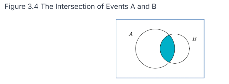
The probability of a union of events P(A⋃B) is the same as either A or B (or both) happening.
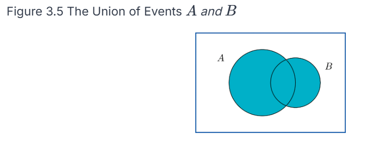
The probability of an intersection of events P(A ⋂ and B) is the same as saying that both A and B happen. We can represent these on a Venn diagram as events (circles) where outcomes are points in each circle. A union would be pictured as both circles shaded in, whereas an intersection would be represented as only the common area being shaded in.
Review
To review, see:
2d. Apply counting rules in the context of combinatorial probability
- What is the definition of a combination, and how is it different from a permutation?
- What are the formulas used to find the number of combinations and the number of permutations?
A combination or permutation refers to the number of possible ways that x out of a possible n outcomes can occur. The difference is that, in a combination, the order does not matter; in a permutation, the order does matter.
For example, there are ten ways to choose x=2 out of the first n=5 letters of the alphabet: AB, AC, AD, AE, BC, BD, BE, CD, CE, and DE. If order does not matter, ten combinations are possible. You could reverse the order of any of the letters, and it would not matter.
There would be 20 permutations if AB and BA were considered different. Without listing them all here, you can intuitively see this because you have ten combinations, and each combination can be in two different orders (AB or BA), so 10×2=20 permutations.
To find the number of ways you can pick r items out of a group of n things, given a permutation, meaning order matters, you use the formula:
!}")
If you are not concerned about the order the items are picked in, you use the formula for combinations:
!\mathrm{r}!}")
Review
To review, see:
2e. Identify common discrete probability distribution functions
- What is a probability distribution, and how does it relate to the frequency tables reviewed in Unit 1?
- What is the difference between a discrete and a continuous probability distribution?
A probability distribution consists of each possible value (or interval of values) of a random variable and the probability that the variable will take on that value.
Probability distributions have many implications in decision-making. When you interpret data, you must know the probability distribution of the value you are trying to estimate. They are related to the frequency tables in that the probabilities are equivalent to the relative frequency distribution.
If you have a list of data, you can get the probabilities on the right side of the table by dividing the frequency by the total number of data points. For example, if the frequency of x=3 is 7 in 20 die rolls, then the probability of rolling a three is 7/20=0.35, so 0.35 would go across from value 3 in the table.
The difference between discrete and continuous probability distributions is analogous to the difference between discrete and continuous variables.
A discrete distribution (like a die roll) has a fixed, finite set of possible values for the random variable x. In contrast, a continuous distribution has many or infinitely many possible values for x. Like a frequency distribution, the values of x must be grouped into intervals. The same rules apply as those that apply to relative frequency histograms: all intervals must be equal in width, non-overlapping, and all-inclusive.
Review
To review, see:
2f. Calculate expected values
- What is the expected value of a distribution, and how is it related to the mean of a set of data?
- What is the formula for expected value?
The expected value of a distribution is another name for the mean of the distribution.
This means that if you take a large set of numbers that follows the original distribution, the arithmetic mean (sum divided by n) of those numbers should roughly equal the expected value of the distribution.
We calculate the value of a distribution by multiplying each value of x by its probability (the median of the interval if it is continuous) and then summing up those numbers.
The formula is ") .
.
This tells us the expected value of x after doing many trials of the experiment.
Review
To review, see:
- Random Variables and Probability Distributions
- Binomial Distributions
- Binomial, Poisson, and Multinomial Distributions
2g. Apply the binomial probability distribution
- What is a binomial experiment?
- What is a binomial distribution?
- What characteristics must a set of events have to follow a binomial distribution?
A binomial experiment is a random experiment that has exactly two possible values (quantitative or qualitative) for x:
- Flipping a coin: x={heads, tails}
- Answer to a true-false question: x={true, false}
- Free throw in basketball: x={made, not made}
A binomial distribution is the distribution of the discrete random variable x, where x represents the number of successes out of n possible events. Note that we mean success in a generic sense: success may not be positive. "Success" means the characteristic you are looking for or researching, regardless of whether you consider the outcome good or bad.
In our basketball free-throw example, if a player takes 10 free-throw shots, they will be successful zero to 10 times. Possible values for x include {0, 1, 2, 3, 4, 5, 6, 7, 8, 9, 10}.
These values and their associated probabilities comprise a binomial probability distribution, which must have three criteria:
- All experiments are binomial.
- All experiments will succeed or fail independently (that is, all free throws are independent events).
- All experiments have an equal probability of success.
A binomial distribution is a family of distributions where each specific distribution consists of two parameters: n is the number of experiments, and p is the probability of success per experiment.
For our basketball example, if the player hits their free throws 75% of the time, we would define this distribution as binomial with n=10 and p=0.75. There are infinite possible binomial distributions, with each combination of n and p making a unique distribution.
Any specific distribution within a family of distributions is defined by its parameters (numerical values determining the particular shape and characteristics of a probability distribution). For example, binomial distributions have parameters n and p. We can calculate the expected value of this distribution by multiplying n and p, or n × p.
Review
To review, see:
2h. Apply the Poisson probability distribution
- What is the definition of a Poisson distribution? When can you use it to estimate a binomial distribution?
- How would you describe a second general use for the Poisson distribution in addition to approximating a binomial distribution?
- A binomial distribution with n=20 and p=0.4 gives the same lambda (or mean) and Poisson distribution as a binomial distribution with n=2000 and p=0.004. How can the same Poisson distribution be "equivalent" to multiple binomial distributions?
The Poisson distribution (pronounced pwah-SOHN or ˈpwɑːsɒn) is related to the binomial distribution because you can use it to approximate the binomial distribution when n is a large value and p is a small value. Unlike the binomial distribution, the Poisson distribution is easier to calculate because it has only one parameter (represented by the Greek letter λ) and the expected value. The calculation is n × p, just as for the binomial distribution.
Statisticians refer to the Poisson distribution as the distribution of rare events. Suppose 1,000 cars drive on a section of road daily, and 1.2 of them get into an accident on average. Since the mean is so small compared to n, we can model this using a Poisson distribution with λ=1.2. We can use the formula to find the probability of x=1 accident, x=2 accidents, and so on.
A minor difference between the Poisson distribution and the binomial distribution is that the binomial distribution is a discrete distribution where all possible values of x are between 0 and n. The Poisson distribution is discrete in that x only has a fixed set of values: in theory, it can have ANY whole number value from 0 to infinity.
For our car example, any probability for x greater than 5 is so remote that it is effectively zero. Theoretically, we could calculate the probability P(x=150).
How would you calculate lambda? x is the expected number of occurrences during a fixed period. So, if a toll booth averages 45 cars per hour, and your fixed period is 10 minutes, then the value of λ would be the expected number in 10 minutes, so 45 per 60 minutes would be 7.5. Note that although they are discrete, the expected value for the binomial and Poisson distributions does not have to be a whole number.
Finally, for each of the two distributions in the third question above, λ=8. However, you should see that finding the probability P(x=7) gives the same answer for two different distributions. The Poisson distribution is a more accurate approximation for the second distribution than for the first. The Poisson distribution is a better predictor of the binomial distribution as n gets larger (and p gets smaller).
Review
To review, see:
2i. Apply continuous probability density functions
- What is the general difference between computing probabilities from discrete vs. continuous distributions?
- What is the explanation of why one rule of continuous probability distributions is that there is zero probability that the random variable x equals any particular value?
In a discrete distribution, we can calculate the probability P(x=x) that x equals a particular value from a formula, depending on the distribution. We can also find probability in a range of values P(1<x<5) by computing P(x=1) through P(x=5) and adding the numbers.
The difference between discrete and continuous distributions is that the probability P(x=x) that x equals a particular value is effectively zero. We can compute P(a<x<b) by finding the area under the density curve between x=a and x=b. It doesn't depend on the height of the graph.
This is why statisticians often call discrete distributions probability distribution functions (mathematical functions that give the probability of each possible outcome for a discrete random variable) and continuous distributions probability density functions. We use the term "density" because probabilities are based on the area between the two numbers, not the height of the graph. A probability density function (a mathematical function that describes the likelihood of a continuous random variable falling within a particular range of values), by definition, has an area of 1 (that is, it is unitless) under the entire curve.
We can explain this rationale in two ways. The most obvious reason is that P(x=x) is a single line, which has no area if we calculate the probability that x is in a range of values by computing the area under the curve. The second reason is more conceptual. Since a continuous distribution has infinite possible values of x, if we are talking about a uniform distribution between x=0 and x=1, an infinite number of numbers exist between those two values. Based on the definition of probability, since there are infinite possible outcomes, 1/∞ tends to 0.
Review
To review, see:
2j. Apply the normal probability distribution
- How can you describe the characteristics of a normal distribution? What sets it apart from any other bell-shaped distribution?
- What does it mean to be symmetric?
- What is the description of a uniform distribution?
- In general, how do we calculate probabilities based on a normal distribution?
- What is the definition of a standard normal distribution,n, and what sets it apart from other normal distributions?
A continuous distribution can be symmetric if the density curve is symmetric around the median, which is also the mean.
A uniform distribution has a flat density curve. Another classic example of this is the discrete distribution, where x is the sum of two six-sided dice. There is only one way each to roll a 2 or a 12, but the median x=7 has six possible ways: {1,6},{2,5},{3,4},{4,3},{5,2},{6,1}. The distribution has higher probabilities toward the mean/median and lower probabilities toward the edges.
A bell-shaped distribution has a bell-shaped density curve, like the dice distribution, except continuous and graphically represented by a smooth curve.
Further in the hierarchy, we have the normal distribution, which has all the characteristics above but with a few additional tell-tale characteristics, which we refer to as the empirical rule:
- The probability of x having a value between one standard deviation below and one standard deviation above the mean is about 68 percent.
- The probability of x being between −2 and +2 standard deviations is about 95 percent.
- The probability of x being between −3 and +3 standard deviations is about 99.7 percent.
There is an important reason why we pluralize "normal distributions" above. As we said earlier, we define distributions by their parameters, such as n and p, for binomial distributions. A given combination of mean  and standard deviation
  makes a particular normal distribution.
Finally, the standard normal distribution is a normal distribution with a mean of 0 and a standard deviation of 1. We will need to obtain a standard normal distribution (often referred to as the z-distribution) to calculate probabilities involving all normal distributions.
To find the probability of x being between a and b in a normal distribution, we must take the following steps:
- Convert the endpoint(s) into z-scores using the formula

- Use technology or a z-distribution table to look up the area to the left of b and the area to the left of a and subtract the two values.
- For p(x < a), convert a into a z-score and find the area left of that value.
- For p(x > b), convert b into a z-score, find the area left of that value, and then subtract that number from 1.
In summary, the hierarchy is:
- Probability distribution
- Continuous probability distribution
- Symmetric
- Normal
- Standard normal (though discrete distributions can also be symmetric)
Review
To review, see:
- The Standard Normal Distribution
- More on Normal Distributions
- Introduction to the Normal Distribution
Unit 2 Vocabulary
This vocabulary list includes terms you will need to know to successfully complete the final exam.
- binomial distribution
- binomial experiment
- combination
- compound event
- conditional probability
- continuous
- continuous distribution
- discrete
- discrete distribution
- empirical rule
- expected value
- intersection
- mutually exclusive
- normal distribution
- parameter
- permutation
- Poisson distribution
- probability
- probability density function
- probability distribution function
- random variable
- standard normal distribution
- uniform distribution
- union
- Venn diagram