MA121 Study Guide
Unit 3: Sampling Distributions
3a. Apply the Central Limit Theorem to approximate sampling distributions
- What is the definition of the sampling distribution of a mean?
- What is the definition of the Central Limit Theorem?
- When can the Central Limit Theorem be applied?
Think again about the difference between sample and population statistics. When you take a sample from a population and measure its sample mean, then take a second sample and measure its mean, and keep going, the set of sample means will have its own distribution. All of these sample means together are called a sampling distribution.
The Central Limit Theorem states that if the original population had a normal distribution, or the sample size is sufficiently large (n=30 as a rule of thumb, but it can be a bit lower if the original population is close to normal), then the sample means themselves will be normally distributed, with a mean  and standard deviation of
  . We often call this standard deviation the standard error.
The Central Limit Theorem can be applied when the sample size is large (generally greater than 30), or when the underlying distribution is normally distributed.
Review
To review, see:
- The Sampling Distribution of a Sample Mean
- The Mean, Standard Deviation, and Sampling Distribution of the Sample Mean
- Sampling Distribution
3b. Describe the role of sampling distributions in inferential statistics
- How does finding probabilities differ for a normal random variable versus the sampling distribution?
- What is the standard error of the mean?
There is a subtle difference between the probabilities we are finding now and those we were seeing at the end of Unit 2. When we learned about probabilities from normal distributions, we solved problems such as: if the population has a mean and standard deviation of 10 and 2, respectively, find the probability that a random variable will have a value between 11 and 14.
The difference here is subtle but important: if the population has a mean and standard deviation of 10 and 2, respectively, find the probability that the mean of a sample of 10 taken from this population will be between 11 and 14.
Another way to think of this is that earlier, you were working with a sample size of n=1, so the above equation for standard error is the same as the population standard deviation since you are dividing by one. So you still find the z-score, but rather than divide by σ, you must divide by (σ/n). The rest of the process is the same: taking those z-scores and using the tables or technology to find the appropriate areas under the curve.
The standard error of the mean is the standard deviation of the sampling distribution of the mean. So, if you have a normal distribution, your sample mean will likely be within this standard error of the population mean.
Review
To review, see:
3c. Interpret a probability distribution for the mean of a discrete variable
- What is the mean of a discrete variable, and how is it similar/different from the mean of a set of numbers?
- How can you create a probability distribution graph for the means of a discrete variable?
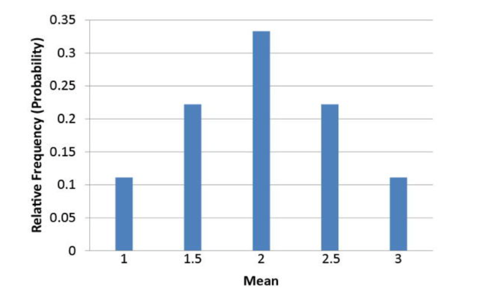
The mean of a discrete random variable (also known as the expected value) is equal to the mean of a set of numbers that comes directly from that discrete distribution. Of course, this assumes no randomness, so the two numbers might be slightly different. Take a very simple discrete distribution: P(X=0)=0.5, P(X=1)=0.2, P(X=5)=0.3. By the rules for the mean of a discrete distribution (see resources below), the mean would be 0.5(0)+0.2(1)+0.3(5)=1.7.
Now, let's take 10 numbers that perfectly represent this distribution: 0, 0, 0, 0, 0, 1, 1, 5, 5, 5. The sum is 17 and 17/10=1.7. So, we get the same number from taking the mean of the distribution versus the mean of numbers from that distribution. Of course, suppose we truly sample from the above distribution. In that case, we will not get those 10 exact numbers because of randomness, so taking the mean of 10 numbers drawn randomly from that distribution will not be exactly 1.7.
We discussed the probability distribution of the means for the averages of the numbers 1, 2, and 3 picked with replacement, two at a time. That graph is shown below.
Review
To review, see:
3d. Describe a sampling distribution in terms of repeated sampling
- What does it mean to take repeated samples from a population?
- What implication does this have?
Taking the means from repeated samples creates a sampling distribution. Doing this enough times allows you to see the many different results produced by different samples from the same population with the same sample size. You can find the probability of x roughly the same way you found the probability of x in Unit 2.
This is important because statistics is ultimately about making predictions about populations based on a sample (inferential statistics). A major step in calculating margins of error is not only to observe the properties of distributions but also to see how the resulting samples behave.
Review
To review, see:
3e. Compute the mean and standard deviation of the sampling distribution of population proportion p and mean
- What is the sampling distribution of a population proportion, and how does it differ from the sampling distribution of a mean?
- How is the process for finding probabilities different? Can we still use the z-distribution?
Similar to the sampling distribution of the mean, you can take repeated samples from a population where p is the proportion having a certain characteristic, and the sample proportions will be normally distributed if the number sampled each time is sufficiently large.
A good rule of thumb is that given the parameters n (sample size) and p (population proportion), we can use the normal distribution if np and n1-pp are both greater than 10 and p is not too close to 0 or 1. With a very small or large value for p, the distribution becomes right- or left-skewed, and finding areas based on the z-score is unreliable.
The mean ( ) and standard deviation (
}}{\sqrt{n}}") ) formulas use the population proportion
) formulas use the population proportion  rather than the sample proportion
  . This becomes an important difference later when you have to make approximations of the population based on samples and do not have access to the population parameters.
Review
To review, see:
3f. Approximate a sampling distribution based on the properties of the population
How do the properties of the population distribution affect the sampling distribution?
If you have a very large sample size, the short answer is that they do not. The sampling distribution will be bell-shaped and have a predictable mean and standard deviation based on the formulas we discussed earlier in the section on learning outcome 3a.
This explanation does not hold for smaller sample sizes where the properties of the sampling distribution are far less predictable. In some cases, we can come up with sampling distributions and properties through small-sample methods, but these examples are beyond the scope of this course.
Review
To review, see:
3g. Compare the sampling distributions of different sample sizes
- What effect does changing the sample size have on the sampling distribution of a mean?
Keep two things in mind here. First, unless the underlying population distribution is normal, the sample size must be sufficiently large for the sampling distribution to be normal. Second, the standard error (standard deviation of the sample means) becomes smaller with a larger sample. More specifically, it decreases by a factor of the square root of the sample size. For example, if you multiply the sample size by 4, you must divide the standard error by 2 (the square root of 4).
Review
To review, see:
Unit 3 Vocabulary
This vocabulary list includes terms you will need to know to successfully complete the final exam.
- Central Limit Theorem
- sampling distribution
- standard error