MA121 Study Guide
Unit 4: Estimation with Confidence Intervals
4a. Compare t-distributions and normal distributions
- What is the difference between a normal distribution and a t-distribution?
- Where would you need to use a t-distribution instead of a normal (x) or the standard normal (z) distribution?
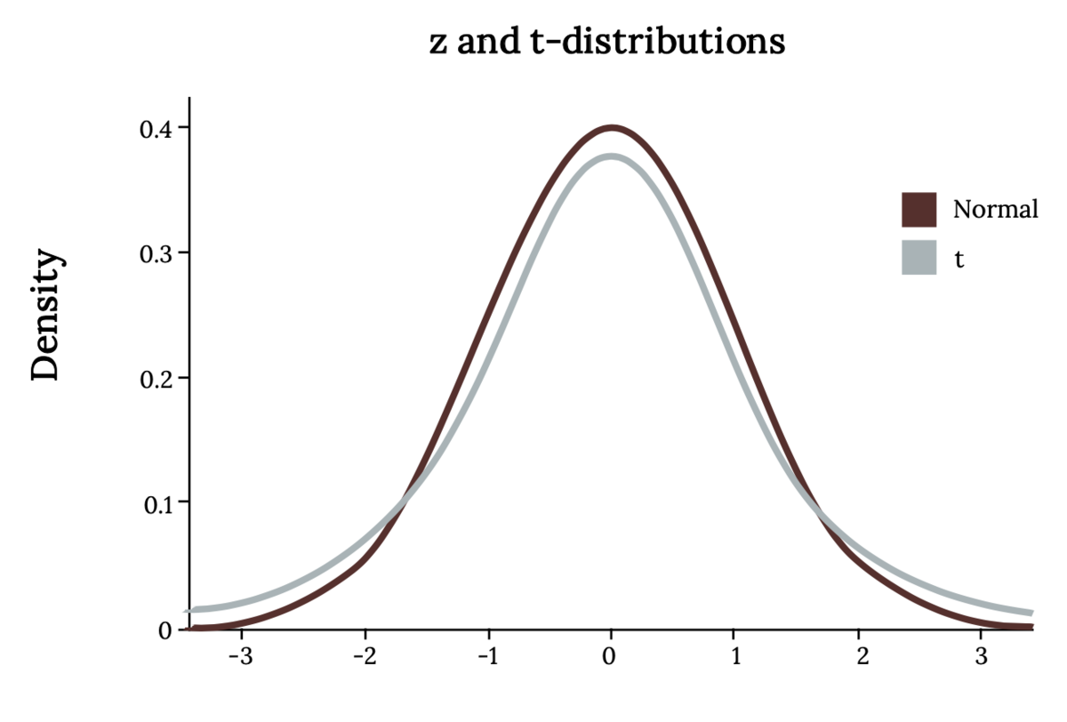
Now, let's introduce the t-distribution, which you can think of as a "brother" to the normal distribution in this hierarchy.
The student's t-distribution is similar to the normal distribution except that it is slightly shorter and flatter, with heavier tails than x or z. In other words, the area to the right of two standard deviations in a normal distribution is 0.025. In a t-distribution, it will be larger. The t-family of distributions is defined by a single parameter called the degrees of freedom, which is symbolized simply as df, although some texts will use other symbols, such as ⋎. When we are talking about the t-distribution, the degrees of freedom are equal to the sample size minus one.
We use the t-distribution in the same situations as the z-distribution. However, we must use t instead when we are unsure of the shape of the population distribution or we are using an estimate of the standard deviation (s instead of σ).
To find an area bound by the t-distribution, we can use technology similar to what we use for the z-distribution. There is a t-distribution table with one row for each of the most common values of t. The drawback is that we cannot use this to find the exact area; only the "t-score" is given for a particular area.
Note that with a t-distribution, as the sample size (thus the degrees of freedom) increases, it is nearly indistinguishable from the z-distribution. In fact, the z-distribution is the t-distribution with an "infinite" degree of freedom! Using the t-distribution gives us a larger margin of error (the range of values above and below a sample statistic that accounts for uncertainty in the estimate) to compensate for the fact that the exact standard deviation of the population is not known.
Review
To review, see:
4b. Describe the performance of different estimators based on their sampling distributions
- What is bias, and how does it differ from accuracy? Can an estimator be biased yet accurate? Can it be inaccurate and unbiased?
- Why is the sample mean considered an unbiased estimator for the population mean?
No estimator is perfect. We use an estimator like a sample mean to give us the best possible estimate of a population mean. However, because of sampling errors, the sample mean will always change for different samples.
Sampling error refers to the fact that, because we do not have access to the entire population, our sample statistics will differ from the population parameters and from each other. If you have a population of size 1,000 with a population mean of 50, you can take five samples of size 20, and because each time you have a different sample, you will get a different sample mean each time, such as {49, 51, 50, 48, 55}.
An unbiased estimator will sometimes estimate too high and sometimes too low, but in the long run, if you average them (the sampling distribution of the mean), you will get a good estimate. In other words, the sample mean is just as likely to overestimate the population mean by 2 as it is to underestimate by 2. A biased estimator might be more likely to overestimate rather than underestimate, or vice versa.
Accuracy differs from bias in that it refers to how much the statistics will differ from the parameter. It's important, but not as much as bias. Accuracy will be better, in general, when we have larger samples, and there is less variance (or standard deviation) in the population.
Review
To review, see:
4c. Calculate confidence intervals for population averages and one population proportion
- What does the confidence interval for a data sample tell you?
- Why was it necessary for you to learn about sampling distributions first?
- How do you calculate a confidence interval?
We use inferential statistics to interpret samples and make conclusions about the population of data. The general method for making these interpretations is roughly the same, whether for population averages, proportions, averages of two different populations, standard deviations, or any other statistic.
Confidence intervals are intervals where we expect to find a population parameter. Think of it as a range of values where we expect the population mean or population proportion to be located. They are calculated at different confidence levels. A 99% confidence interval would have a larger interval, while a 90% confidence interval would be smaller.
First, we find a point estimate, which is usually the sample mean or proportion. Then, given the level of confidence desired, the sample size, and the standard deviation of the population, we can find a margin of error and subtract or add it to the point estimate to get a confidence interval for the population parameter.
When we refer to the level of confidence, we mean the likelihood that our confidence interval contains the true population mean or proportion (or other parameter). Common confidence levels are 90%, 95%, and 99%. A higher confidence level gives a higher likelihood that the interval contains the population parameter. However, the price to be paid is that a higher confidence interval will naturally be wider.
So, for example, we could say there is a 95 percent probability that the population mean is between 10 ± 2.8, or [7.2, 10.8]. If we want to be 99 percent confident, we have to increase the width of the interval, perhaps to 10 ± 3.2. A 100 percent confidence interval is impossible since that would require an infinitely wide margin of error. So there is a give and take. Choosing a confidence level can be more art than science. Balance your desire for accuracy with the need to keep the margin of error low.
You had to learn about sampling distributions first because inferential statistics involves predicting the characteristics of a population based on a sample. To do so, we must first study how those samples behave.
Use the given formulas to calculate the margin of error for the population mean, given a large population (this is when you use the standard normal z-distribution). If the population is small or large and the standard deviation of the population is unknown, you must use Student's t.
The formulas are very similar, except for the distribution. You would use the inverse z-distribution or inverse t-distribution with given degrees of freedom. You also have to plug in the z- or t-score corresponding to ∝/2, where ∝ is equal to the tail area on one side. For example, if you are trying to find a 90 percent confidence interval, that will leave a 10 percent area on the tails, which you divide in half to come up with ∝/2=0.10/2=0.05.
Review
To review, see:
- Basic Sample Statistics and Parameters
- Confidence Interval Simulation
- Confidence Intervals for Correlation and Proportion
4d. Interpret the student-t probability distribution as the sample size changes
- How is the student's t-distribution related to sample size? Why does this not matter for normal or standard normal distributions?
- What happens to the student's t-distribution as the sample size increases? What distribution does it begin to resemble?
The student's t-distribution, like the normal distribution, is a family of distributions defined by one or more parameters. A normal distribution is defined by its mean and standard deviation. The student's t-distribution is defined by the number of degrees of freedom, which is equal to the sample size minus 1.
The larger the sample size, the lower the margin of error, and the larger the degrees of freedom, which combined will give you a smaller margin of error. The larger the degrees of freedom, the more the t-distribution resembles the standard normal (z) distribution. A z-distribution is, by definition, the same as a t-distribution with infinite degrees of freedom!
Review
To review, see:
Unit 4 Vocabulary
This vocabulary list includes terms you will need to know to successfully complete the final exam.
- accuracy
- biased estimator
- confidence interval
- degrees of freedom
- level of confidence
- margin of error
- point estimate
- sampling error
- student's t-distribution
- unbiased estimator